Interactive object clustering#
In this exercise we will use the napari-clusters-plotter to group objects together based on their measured properties. For these measurements we will use napari-skimage-regionprops.
Starting point#
Open a terminal window and activate your conda environment:
conda activate devbio-napari-env
Afterwards, start up Napari:
napari
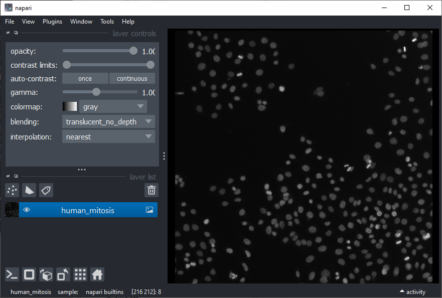
In Napari open the “Human mitosis” example dataset from the menu File > Open Sample > Napari builtins > Human mitosis.
Object segmentation#
Segment the nuclei using the menu Tools > Segmentation / Labeling > Gauss-Otsu Labeling (clesperanto).
Keep the default settings and click Run.
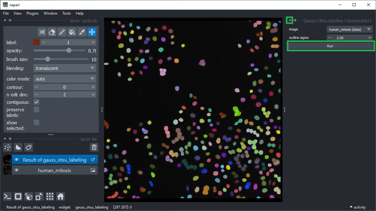
Use the small hide icon to close the Gauss-Otsu-Labeling widget.
Feature extraction#
Measure shape and intensity features using the menu Plugins > Measurement Tables > Regionprops (scikit-image, nsr).
Make sure that the intensity, size and shape checkboxes are ticked and click Run.
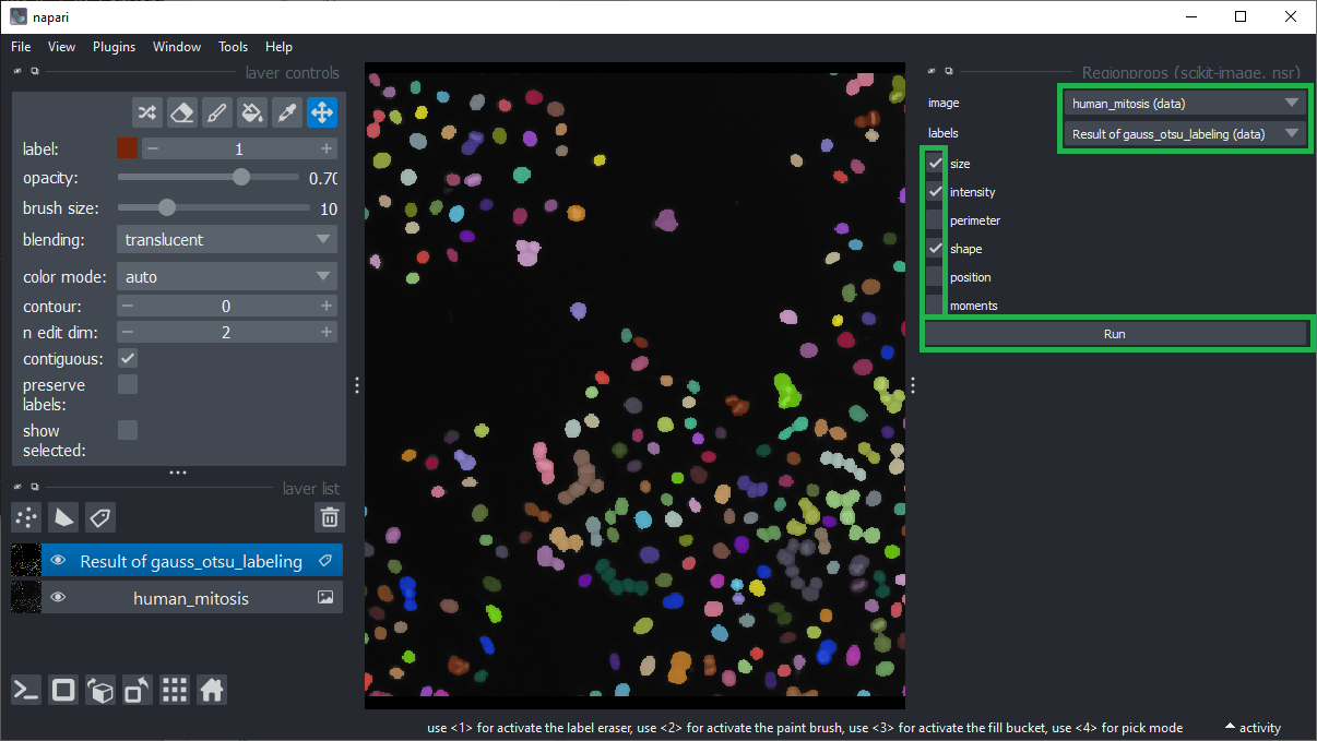
Hide both, the Regionprops widget and the Table widget that just popped up.
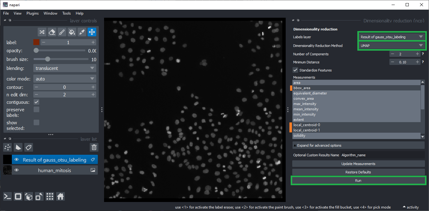
Dimensionality reduction#
Generate a UMAP using the menu Plugins > Measurement post-processing > Dimensionality Reduction > UMAP (nsr).
Make sure the labels layer is selected where you just did your measurements.
Choose the method
UMAPand keep its default settings.Untick the features
bbox_area, andlocal_centroid1/2using theCTRLkey.Click
Run.Wait a minute.
Close both, the Dimensionality Reduction widget and the Table widget that just popped up.
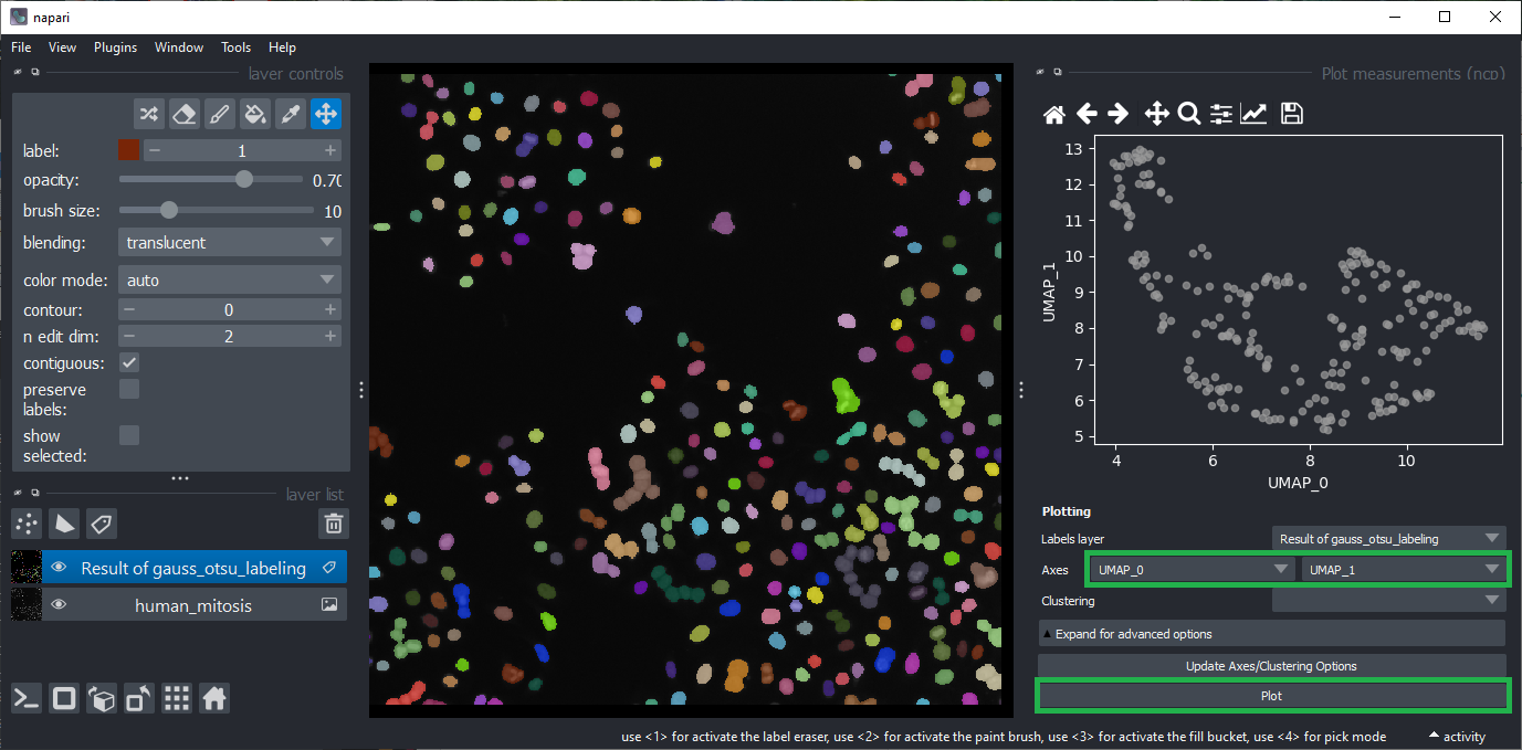
Plot measurements#
Open the plot widget using the menu Plugins > Visualization > Plot measurements (ncp).
You can play a bit with columns to plot. Eventually select UMAP_0 and UMAP_2 as Axes and click on Plot.
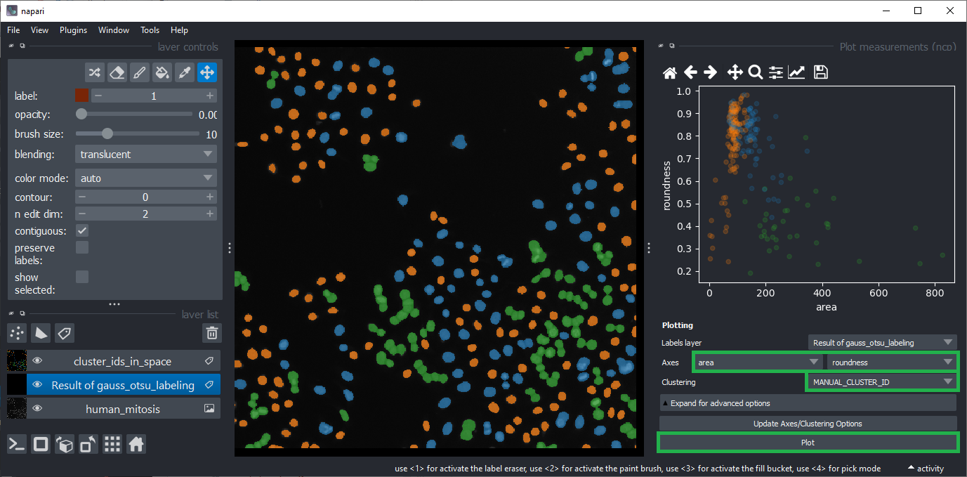
Manual clustering#
Click within the plot and before releasing the mouse button, drag the mouse to select a region of interest.
Repeat this while holding the CTRL key to select multiple regions of interest.
The object selection might be related to their shape and size.
To visualize this hypothesis, you can select the area and roundness as Axes in the plot widget.
Make also sure the clustering MANUAL_CLUSTER_ID is selected.
Click on Plot again.
Close the plot widget.
Automatic clustering#
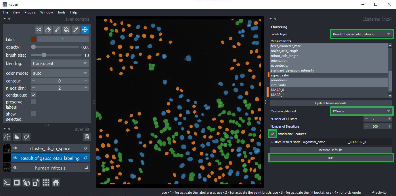
You can also cluster the objects automatically using the menu Plugins > Measurement post-processing > Clustering (nsr) menu.
Choose the layer of the segmented and measured objects.
Unselect the bbox_area and local_centroid1 / 2 features.
Unselect aspect_ratio because it sometimes contains inf values which are not supported by the clustering algorithm.
Also unselect UMAP_0 and UMAP_1 as these two contain compressed information about all other columns.
Select K-Means clustering and activate the Standardize features checkbox.
Click on Run.
Close the Clustering widget and the Table widget that just popped up.
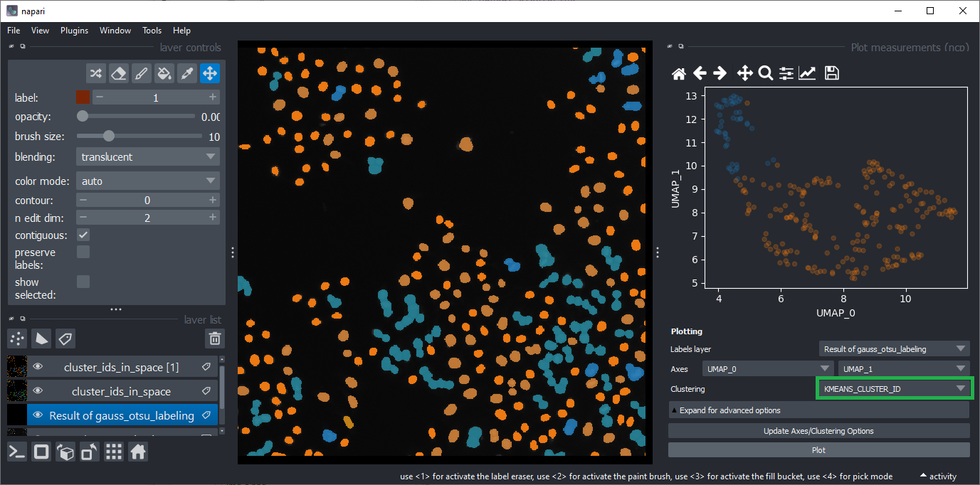
Visualizing automatic clustering#
To visualize the results of the automated clustering, open the plot widget again using the menu Plugins > Visualization > Plot measurements (ncp).
Select UMAP_0 and UMAP_1 as Axes and select KMEANS_CLUSTER_ID as Clustering.
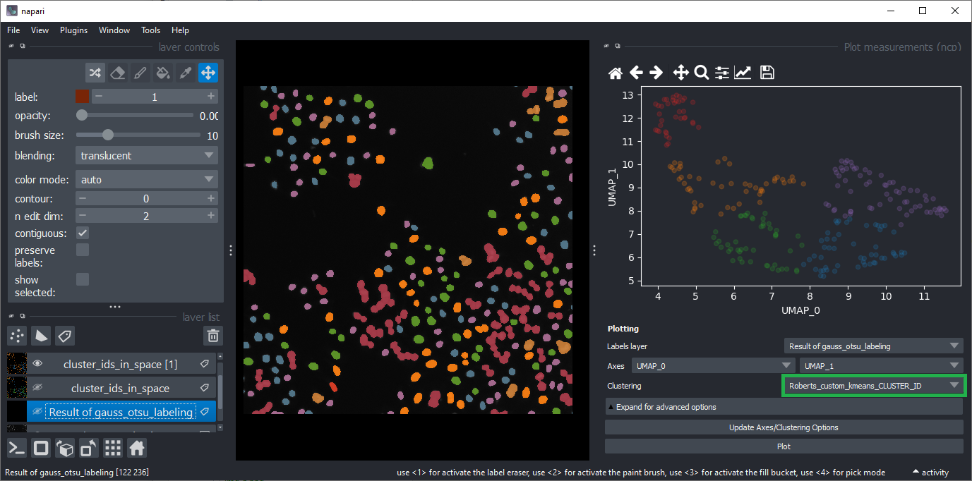
Exercise#
Cluster the objects into 5 classes while having only UMAP_0 and UMAP_1 selected in the Clustering widget.
Give this clustering result a name.
Visualize the resulting clustering using the plot widget.
The result should approximately look like this: