Generating code using bia-bob

BIA Bob is a Jupyter-magic based assistant for interacting with data via code generation. We can initialize it to use the ScaDS.AI LLM server like this:

import os
from bia_bob import bob
bob.initialize(endpoint="https://llm.scads.ai/v1",
               api_key=os.environ.get('SCADSAI_API_KEY'), 
               model="meta-llama/Llama-3.3-70B-Instruct")

This notebook may contain text, code and images generated by artificial intelligence. Used model: meta-llama/Llama-3.3-70B-Instruct, vision model: None, endpoint: https://llm.scads.ai/v1, bia-bob version: 0.25.3.. Do not enter sensitive or private information and verify generated contents according to good scientific practice. Read more: https://github.com/haesleinhuepf/bia-bob#disclaimer

You can use the %bob single-line or the %%bob multi-line magic to ask for programming image analysis tasks and bob will do it for you.

%bob Load the blobs.tif image file and show it.

import skimage.io
import stackview

image = skimage.io.imread("blobs.tif")
stackview.insight(image)

shape (254, 256) dtype uint8 size 63.5 kB min 8 max 248

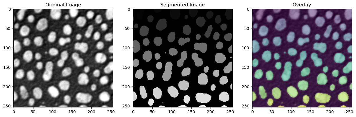
%%bob
Load the blobs.tif grayscale image from disc.
Segment the nuclei-like objects in it using 
Otsu's method and connected component labeling.
Visualize the result next to the original and 
also visualize an overlay of both images

import matplotlib.pyplot as plt
import numpy as np
from skimage.io import imread
from skimage.filters import threshold_otsu
from skimage.measure import label

# Load the image
new_image = imread("blobs.tif")

# Apply Otsu's thresholding
new_threshold = threshold_otsu(new_image)
new_binary_image = new_image > new_threshold

# Apply connected component labeling
new_labels = label(new_binary_image)

# Create a figure with three subplots
fig, axs = plt.subplots(1, 3, figsize=(15, 5))

# Visualize the original image
axs[0].imshow(new_image, cmap='gray')
axs[0].set_title('Original Image')

# Visualize the segmented image
axs[1].imshow(new_labels, cmap='gray')
axs[1].set_title('Segmented Image')

# Visualize an overlay of both images
axs[2].imshow(new_image, cmap='gray')
axs[2].imshow(new_labels, cmap='viridis', alpha=0.5)
axs[2].set_title('Overlay')

plt.show()

Exercise

Ask bob to solve a task in another scientific domain.

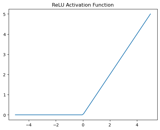
%bob draw a plot of a ReLU Activation function. Keep it short.

import numpy as np
import matplotlib.pyplot as plt

x_values = np.linspace(-5, 5, 100)
y_values = np.maximum(x_values, 0)
plt.plot(x_values, y_values)
plt.title('ReLU Activation Function')
plt.show()