Time Series Analysis with AutoML - Time Series Analysis

This notebook demonstrates AutoML-based time series forecasting using AutoGluon. AutoGluon automatically trains and compares multiple models from classical statistical methods to deep learning and combines the best ones into a weighted ensemble.

What you will see:

How to wrap data into AutoGluon’s TimeSeriesDataFrame
How to configure and train a TimeSeriesPredictor
How to compare model performance via the leaderboard
How to generate and visualize multi-step forecasts

When to use AutoML:

You need a strong baseline quickly without manually tuning individual models
You want to benchmark multiple model families at once
You have limited domain knowledge about which model class suits your data

Pitfall: AutoML hides complexity but does not eliminate it. Always inspect the leaderboard, check that the inferred frequency is correct, and validate that the prediction horizon (prediction_length) matches your real use case.

import pandas as pd
from matplotlib import pyplot as plt
from autogluon.timeseries import TimeSeriesDataFrame, TimeSeriesPredictor

import warnings
warnings.filterwarnings("ignore")

Load Data¶

We use the same DWD weather dataset, resampled to weekly means. The data is split at end of 2022, everything up to that point is used for training; the remaining ~2 years serve as the hold-out period we want to predict.

An id_column with a constant value is added because AutoGluon requires a panel-data format even for a single time series. Each row must belong to an identified series.

df = pd.read_csv("data/dwd_02932_climate.csv", sep=";", parse_dates=["date"], index_col="date")[["temperature_air_mean_2m", "precipitation_height", "pressure_vapor", "humidity"]].resample("W").mean()
df['id_column'] = 'weather'
df.info()

<class 'pandas.core.frame.DataFrame'>
DatetimeIndex: 2610 entries, 1975-01-05 to 2025-01-05
Freq: W-SUN
Data columns (total 5 columns):
 #   Column                   Non-Null Count  Dtype  
---  ------                   --------------  -----  
 0   temperature_air_mean_2m  2610 non-null   float64
 1   precipitation_height     2610 non-null   float64
 2   pressure_vapor           2610 non-null   float64
 3   humidity                 2610 non-null   float64
 4   id_column                2610 non-null   object 
dtypes: float64(4), object(1)
memory usage: 122.3+ KB

df.loc[:"2022"].tail()

Create TimeSeriesDataFrame¶

TimeSeriesDataFrame is AutoGluon’s internal container for time series data. It requires:

A timestamp_column with regular datetime values
An id_column identifying each individual series (required even for a single series)
All remaining numeric columns are treated as the target or covariates

Pitfall: AutoGluon distinguishes between past covariates (known only up to the forecast origin) and known covariates (available in the future). Features like precipitation are past covariates here, they are not known ahead of time and cannot be used to improve future predictions unless a separate forecast is provided for them.

train_data = TimeSeriesDataFrame.from_data_frame(
    df.loc[:"2022"].reset_index(),
    id_column="id_column",
    timestamp_column="date"
)
train_data.tail()

Configure the Predictor¶

Key parameters:

prediction_length: number of future steps to forecast. Here 104 = 2 years of weekly data. Choose this based on your actual forecasting horizon, setting it too large forces models to extrapolate far and degrades accuracy.
target: the column to forecast, all other numeric columns become covariates.
eval_metric: MASE (Mean Absolute Scaled Error) is scale-independent and handles seasonality well. It compares model error against a naive seasonal baseline, a score below 1.0 means the model beats the naive forecast.
random_seed: fixes randomness for reproducibility across runs.

Pitfall: The path argument determines where trained models are saved to disk. If you re-run without deleting this folder, AutoGluon will load cached models instead of retraining.

predictor = TimeSeriesPredictor(
    prediction_length=104,
    path="autogluon-weather-forecast",
    target="temperature_air_mean_2m",
    eval_metric="MASE",
)

Train with AutoGluon¶

predictor.fit() trains all candidate models within the given time_limit and then fits a WeightedEnsemble on top. The presets parameter controls the trade-off between quality and speed:

Preset	Models	Use case
`fast_training`	lightweight statistical and tree-based models only	quick baseline
`medium_quality`	models from fast + plus deep learning models	balanced
`high_quality`	mix of multiple DL, ML and statistical forecasting models	higher accuracy, longer training
`best_quality`	same as high + validation with multiple backtests	production

What happens internally:

Models are trained sequentially, each receiving a time budget proportional to remaining time.
Validation is done on the last prediction_length steps of the training set (rolling window).
Models that exceed their time budget are skipped.
A WeightedEnsemble is fitted last, combining model predictions by minimizing validation error.

Pitfall: Deep learning models (TFT, DeepAR, Chronos) dominate training time. With time_limit=600, simpler models finish in seconds while neural models may each consume 100+ seconds. If time is tight, use presets="medium_quality" or explicitly pass hyperparameters to restrict the model set.

predictor.fit(
    train_data,
    presets="high_quality",
    time_limit=600,
)

Leaderboard¶

The leaderboard ranks all trained models by their validation score (higher = better; scores are negated MASE, so closer to 0 is better). Key columns:

score_val: validation MASE (negated). A value of −0.83 means MASE = 0.83, better than the seasonal naive baseline.
pred_time_val: inference time in seconds, relevant for production latency constraints.
fit_time_marginal: training time for that model alone.

Reading the results: The WeightedEnsemble typically wins or ties the best individual model. If a simple model like DirectTabular is close to the ensemble, the added complexity of deep learning may not be worth it for your use case.

Pitfall: Leaderboard scores are evaluated on the last prediction_length steps of the training set, not on truly unseen data. Always validate on a separate hold-out set before drawing conclusions.

lb = predictor.leaderboard()
lb

Generate Forecasts¶

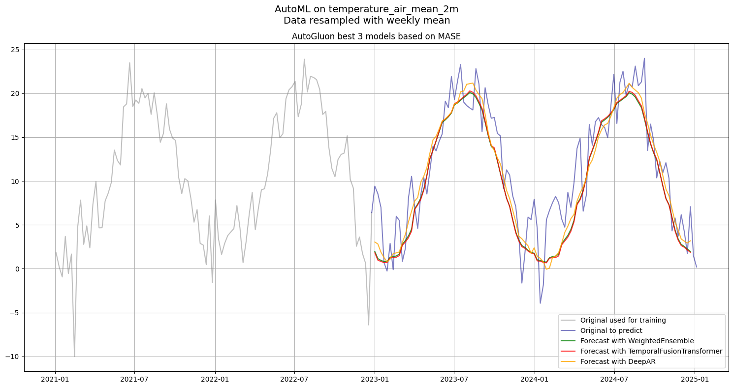
predictor.predict() returns a TimeSeriesDataFrame with quantile forecasts (0.1–0.9) plus the mean prediction. Here we extract only the mean for the top 3 models from the leaderboard to compare them visually.

Pitfall: predictor.predict() always forecasts the next prediction_length steps after the last timestamp in the input data. If you pass the full training set, forecasts start at 2023-01-01. Make sure your input data ends exactly where you want the forecast to begin.

predictions = {}
for model in lb["model"][:3]:
    predictions[model] = predictor.predict(train_data, model=model).to_data_frame().reset_index()[["timestamp", "mean"]].set_index("timestamp")

plt.figure(figsize=(15, 8))
plt.plot(df["temperature_air_mean_2m"].loc["2021":"2022"], label='Original used for training', color='grey', alpha=0.5)
plt.plot(df["temperature_air_mean_2m"].loc["2022-12-25":], label='Original to predict', color='darkblue', alpha=0.5)
for (model, pred), color in zip(predictions.items(), ['green', 'red', 'orange']):
    plt.plot(pred, label=f'Forecast with {model}', alpha=0.8, color=color)
plt.suptitle(f"AutoML on {df["temperature_air_mean_2m"].name}\nData resampled with weekly mean", fontsize=14)
plt.title("AutoGluon best 3 models based on MASE", fontsize=12)
plt.legend()
plt.grid(True)
plt.tight_layout()
plt.show()