Time Series Analysis - Traditional Methods - Time Series Analysis

This notebook demonstrates classical statistical approaches to time series forecasting and anomaly detection using meteorological data.

Methods covered:

Anomaly detection: Z-Score on residuals, IQR detector
ARIMA family: AR, MA, ARMA, SARIMA, AutoARIMA
Exponential Smoothing: Holt-Winters (additive trend + seasonality)
State Space Models: Kalman filter with and without covariates

All forecasting targets weekly mean temperature (temperature_air_mean_2m), trained on 1975–2022 and evaluated on 2023–2024.

import pandas as pd
import matplotlib.pyplot as plt
import seaborn as sns
from darts import TimeSeries

import warnings
from statsmodels.tools.sm_exceptions import InterpolationWarning
warnings.simplefilter('ignore', InterpolationWarning)
warnings.filterwarnings('ignore', category=FutureWarning)

Load Data¶

df_full = pd.read_csv("data/dwd_02932_climate.csv", sep=";", parse_dates=["date"], index_col="date")
df_full.info()

<class 'pandas.core.frame.DataFrame'>
DatetimeIndex: 18263 entries, 1975-01-01 to 2024-12-31
Data columns (total 14 columns):
 #   Column                     Non-Null Count  Dtype  
---  ------                     --------------  -----  
 0   wind_gust_max              18006 non-null  float64
 1   wind_speed                 18240 non-null  float64
 2   precipitation_height       18263 non-null  float64
 3   precipitation_form         18263 non-null  float64
 4   sunshine_duration          18082 non-null  float64
 5   snow_depth                 18233 non-null  float64
 6   cloud_cover_total          18263 non-null  float64
 7   pressure_vapor             18263 non-null  float64
 8   pressure_air_site          18263 non-null  float64
 9   temperature_air_mean_2m    18263 non-null  float64
 10  humidity                   18263 non-null  float64
 11  temperature_air_max_2m     18263 non-null  float64
 12  temperature_air_min_2m     18263 non-null  float64
 13  temperature_air_min_0_05m  18263 non-null  float64
dtypes: float64(14)
memory usage: 2.1 MB

For further analysis and forecasting, we select a subset of variables showing a high correlation with “temperature_air_mean_2m”.

We also include “precipitation_height” for outlier analysis.

df = df_full[["temperature_air_mean_2m", "precipitation_height", "pressure_vapor", "humidity"]]
df.info()

<class 'pandas.core.frame.DataFrame'>
DatetimeIndex: 18263 entries, 1975-01-01 to 2024-12-31
Data columns (total 4 columns):
 #   Column                   Non-Null Count  Dtype  
---  ------                   --------------  -----  
 0   temperature_air_mean_2m  18263 non-null  float64
 1   precipitation_height     18263 non-null  float64
 2   pressure_vapor           18263 non-null  float64
 3   humidity                 18263 non-null  float64
dtypes: float64(4)
memory usage: 713.4 KB

The dataset is loaded with 4 variables, all complete (no missing values at the daily level).

Train / test split strategy:

Training: 1975–2022
Test (forecast horizon): 2023–2024

Pitfall:
The split must be strictly temporal without shuffling.
Any data from the test period used during fitting (even for scaling or feature engineering) constitutes data leakage and will produce optimistically biased evaluation metrics.

Anomaly Detection¶

Detecting outliers before modelling is important: a single extreme value can distort model parameters significantly, especially in small-window calculations (moving averages, ACF estimates).

Two complementary approaches are shown:

Z-Score on residuals: Deviation from the STL residual mean in standard deviations, assumes that residuals are roughly normal distributed
IQR detector: Points outside [Q1 − scale×IQR, Q3 + scale×IQR], Non-parametric, no distributional assumption

Pitfalls:
Z-Score: Applying Z-Score directly to a seasonal series (without decomposing first) flags seasonal peaks as anomalies. Always decompose and score the residuals, not the raw series.
IQR: IQR is applied to the raw series here. For variables with strong seasonality, the interquartile range spans seasonal variation — the detector may miss genuine outliers in low-variance seasons.

Z-Score¶

Anomaly Detection with Z-Score on Residuals

from statsmodels.tsa.seasonal import STL
from scipy.stats import zscore

df_prec = df[['precipitation_height']].copy()

# Extract residuals
df_prec['residuals'] = STL(df_prec, period=365).fit().resid

# Calculate z-scores for the residuals
df_prec['z_scores'] = zscore(df_prec['residuals'])

# Define a threshold for anomaly detection
z_score_threshold = 3  # Common threshold for detecting anomalies
df_prec['outliers'] = df_prec['z_scores'].abs() > z_score_threshold

fig, ax = plt.subplots(2, 1, figsize=(20, 15))
# Plot residuals with marked outliers
sns.scatterplot(data=df_prec, x=df_prec.index, y='residuals', hue='outliers', size='z_scores', 
                palette={True: 'red', False: 'blue'}, legend="brief", ax=ax[0])
# Plot timeseries with marked outliers
sns.lineplot(data=df_prec, x=df_prec.index, y='precipitation_height', alpha=0.5, ax=ax[1])
sns.scatterplot(x=df_prec.index[df_prec['outliers']], y=df_prec['precipitation_height'][df_prec['outliers']], 
                color='red', label='Outliers', ax=ax[1])
plt.suptitle('Anomaly Detection on Residuals for Z-Score > 3', fontsize=14)
plt.show()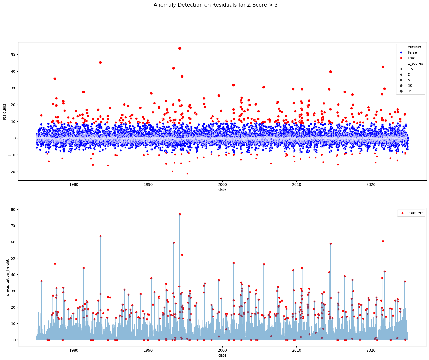

IQR Detector with darts¶

IQRDetector from darts implements the same IQR logic as a reusable fitted object that works directly with TimeSeries. The scale parameter multiplies the IQR to set how wide the non-anomaly band is (default = 1.5 as in Tukey’s rule; scale=3 is more conservative).

Pitfall:
fit_detect fits the IQR bounds on the same data it detects. This is appropriate for exploratory analysis but not for a production pipeline where bounds should be fit on training data only, then applied to new data with .detect().

from darts.ad.detectors.iqr_detector import IQRDetector

series_prec = df['precipitation_height'].copy()

iqr_detector = IQRDetector(scale=3).fit_detect(TimeSeries.from_series(series_prec))
iqr_outliers = iqr_detector.to_dataframe().rename(columns={'precipitation_height': 'outliers'})['outliers'].astype('bool')

fig, ax = plt.subplots(figsize=(20, 7))
# Plot timeseries with marked outliers
sns.lineplot(x=series_prec.index, y=series_prec, alpha=0.5, ax=ax)
sns.scatterplot(x=series_prec.index[iqr_outliers], y=series_prec[iqr_outliers], color='red', label='Outliers', ax=ax)
plt.suptitle('Anomaly Detection with darts IQR', fontsize=14)
plt.show()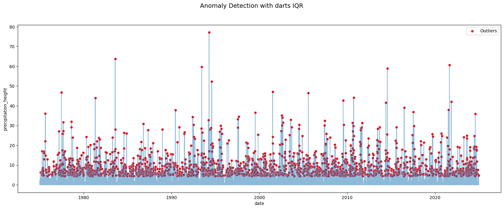

Modeling and Forecasting with ARIMA Model Family¶

The ARIMA family models a time series using its own past values and past forecast errors:

Model	Parameters	What it captures
AR(p)	`p` lags	Autocorrelation - past values predict future values
MA(q)	`q` lags	Error smoothing - past forecast errors correct future predictions
ARMA(p,q)	`p`, `q`	Both simultaneously
ARIMA(p,d,q)	`p`, `d`, `q`	ARMA + `d` rounds of differencing to remove trend/non-stationarity
SARIMA(p,d,q)(P,D,Q,s)	+ seasonal terms	Seasonal AR, MA, and differencing at period `s`

Choosing p, q: ACF/PACF plots below guide order selection - PACF cuts off at lag p (AR), ACF cuts off at lag q (MA).

Pitfall:
ARIMA assumes the series is (or can be made) stationary after d differences.
Seasonal patterns must be handled explicitly via SARIMA or prior decomposition, plain ARIMA on a seasonal series will produce poor forecasts.

We will use weekly resampled data for faster computation.

from statsmodels.tsa.ar_model import AutoReg
from statsmodels.tsa.arima.model import ARIMA
from statsmodels.tsa.statespace.sarimax import SARIMAX

df_w = df.resample("W").mean()
df_w.info()

<class 'pandas.core.frame.DataFrame'>
DatetimeIndex: 2610 entries, 1975-01-05 to 2025-01-05
Freq: W-SUN
Data columns (total 4 columns):
 #   Column                   Non-Null Count  Dtype  
---  ------                   --------------  -----  
 0   temperature_air_mean_2m  2610 non-null   float64
 1   precipitation_height     2610 non-null   float64
 2   pressure_vapor           2610 non-null   float64
 3   humidity                 2610 non-null   float64
dtypes: float64(4)
memory usage: 102.0 KB


df_w_temp = df_w['temperature_air_mean_2m']

df_w_temp_train = df_w_temp.loc[:'2022']

print(df_w_temp_train.tail())

date
2022-11-27    3.614286
2022-12-04    1.714286
2022-12-11    0.600000
2022-12-18   -6.414286
2022-12-25    6.400000
Freq: W-SUN, Name: temperature_air_mean_2m, dtype: float64

Order Selection via ACF / PACF¶

Before fitting any ARIMA-family model, inspect the ACF and PACF of the training series to guide p and q selection:

PACF cuts off sharply at lag p, ACF decays slowly: AR(p)
ACF cuts off sharply at lag q, PACF decays slowly: MA(q)
Both decay slowly: ARMA(p, q), try small values of both

The ACF/PACF are plotted here on the full series (including test) for visual clarity, but in practice order selection should use training data only to avoid lookahead bias.

from darts.utils.statistics import plot_acf, plot_pacf

# Iterate over each column to plot ACF and PACF
fig, (ax1, ax2) = plt.subplots(nrows=1, ncols=2, figsize=(12, 4))
plot_acf(TimeSeries.from_series(df_w_temp), max_lag=60, alpha=0.05, axis=ax1)
plot_pacf(TimeSeries.from_series(df_w_temp), max_lag=60, alpha=0.05, axis=ax2)
plt.suptitle(f'ACF and PACF for {df_w_temp.name}')
plt.tight_layout()
plt.show()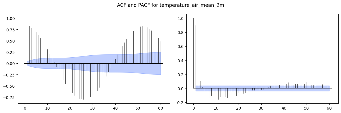

p = 1
q = 3

Auto Regression (AR)¶


ar_model = AutoReg(df_w_temp_train, lags=p).fit()

Moving Average (MA)¶


ma_model = ARIMA(df_w_temp_train, order=(0, 0, q)).fit()

Autoregressive Moving Average (ARMA) - ARIMA with d=0 (no differencing)¶


arma_model = ARIMA(df_w_temp_train, order=(p, 0, q)).fit()

Seasonal Autoregressive Integrated Moving-Average (SARIMA)¶

P = 1
Q = 1
s = 52
sarima_model = SARIMAX(df_w_temp_train, order=(p, 0, q), seasonal_order=(P, 0, Q, s)).fit()

Generating Predictions¶

predict(start, end) with integer indices covers both:

In-sample fitted values (start within training): shows how well the model fits the data it was trained on; this is not a measure of forecast quality
Out-of-sample forecasts (end beyond training): the genuine test of generalization

The plot shows only 2021 onwards for visual clarity, but the models were trained on the full 1975–2022 history.

Pitfall:
In-sample fit is almost always better than out-of-sample performance.
A model that looks perfect on the training window (e.g. SARIMA with many parameters) may still forecast poorly, always evaluate on held-out data.

start = len(df_w_temp.index) - 208
end = len(df_w_temp.index) - 1
ar_pred = ar_model.predict(start=start, end=end)
ma_pred = ma_model.predict(start=start, end=end)
arma_pred = arma_model.predict(start=start, end=end)
sarima_pred = sarima_model.predict(start=start, end=end)

plt.figure(figsize=(15, 8))
plt.plot(df_w_temp.loc["2021":"2023"], label='Original used for training', color='grey', alpha=0.5)
plt.plot(df_w_temp.loc["2023":], label='Original to predict', color='darkblue', alpha=0.5)
plt.plot(ar_pred.loc["2021":], label=f'Modelled with AR(p={p})', color='orange')
plt.plot(ma_pred.loc["2021":], label=f'Modelled with MA(q={q})', color='green')
plt.plot(arma_pred.loc["2021":], label=f'Modelled with ARMA(p={p},q={q})', color='red')
plt.plot(sarima_pred.loc["2021":], label=f'Modelled with SARIMA(p={p},q={q})(P={P},Q={Q},s={s})', color='purple')
plt.title(f"Auto Regression and Moving Averages on {df_w_temp.name} \nData resampled with weekly mean", fontsize=14)
plt.legend()
plt.grid(True)
plt.show()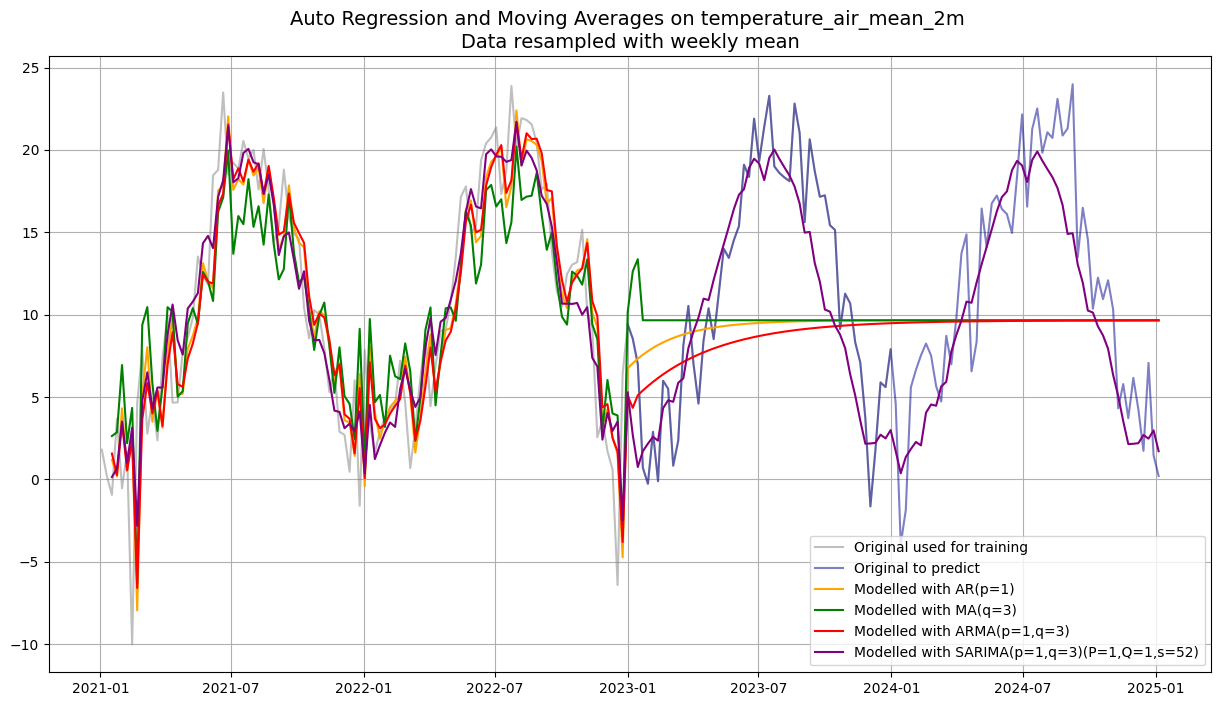

AutoARIMA - Automated Order Selection¶

AutoARIMA wraps pmdarima.auto_arima, which performs a stepwise search over (p, d, q) and seasonal (P, D, Q) combinations, selecting the model with the lowest AIC (Akaike Information Criterion) by default.

Advantages over manual selection:

Automatically determines the differencing order d via unit-root tests
Tests seasonal and non-seasonal components together
Deterministic and reproducible

Pitfall:
AutoARIMA can be slow on long series with many seasonal candidates.
AIC minimisation does not guarantee best forecast accuracy, it penalises complexity but can still overfit.
Validate on the held-out test set regardless of the AIC-selected order.

from darts.models import AutoARIMA

temp_series_train = TimeSeries.from_series(df_w_temp_train)

autoarima_model = AutoARIMA(season_length=52)
autoarima_model.fit(temp_series_train)

autoarima_pred = autoarima_model.predict(104)

plt.figure(figsize=(15, 8))
plt.plot(df_w_temp.loc["2021":"2022"], label='Original used for training', color='grey', alpha=0.5)
plt.plot(df_w_temp.loc["2022-12-25":], label='Original to predict', color='darkblue', alpha=0.5)
plt.plot(autoarima_pred.to_series(), label='Modelled with AutoARIMA(season_length=52)', color='red')
plt.title(f"AutoML with darts AutoARIMA on {df_w_temp.name} \nData resampled with weekly mean", fontsize=14)
plt.legend()
plt.grid(True)
plt.show()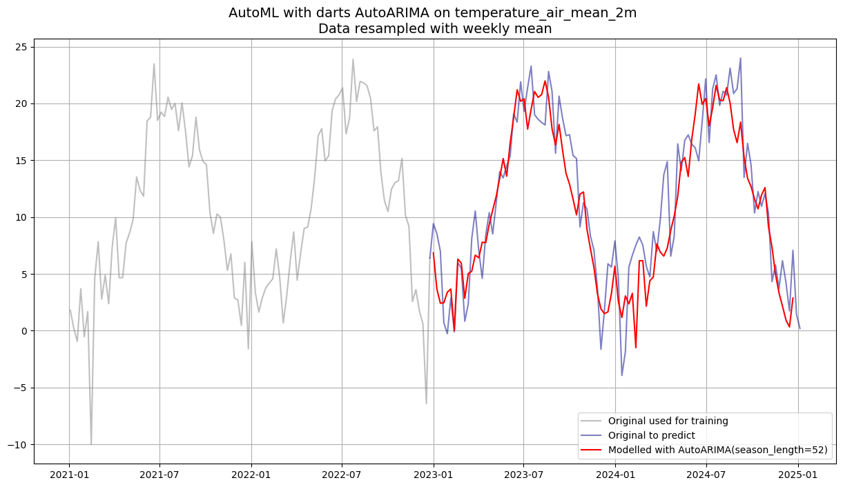

Exponential Smoothing with Holt-Winters¶

Exponential smoothing models predict future values as a weighted average of past observations, where more recent observations receive higher weight. There are three levels of complexity:

Model	Components	Parameters
Simple (SES)	Level only	`α`
Double (Holt)	Level + Trend	`α`, `β`
Triple (Holt-Winters)	Level + Trend + Seasonality	`α`, `β`, `γ`

Additive vs multiplicative seasonal:

Additive: seasonal fluctuation is constant in magnitude - suitable here (temperature amplitude is stable)
Multiplicative: fluctuation grows with the level - typical for economic/sales data

Normally the smoothing weights are optimised via MLE. Here smoothing_trend and smoothing_seasonal are fixed at 0.4 to demonstrate the effect of a specific weighting.

Pitfall:
Manually fixing smoothing weights prevents the model from adapting to the actual data dynamics.
A weight of 0.4 is quite high (strong recency bias) and may cause instability over a 2-year forecast horizon.
Let the model optimise the weights for production use.

from darts.models.forecasting.exponential_smoothing import ExponentialSmoothing
from darts.utils.utils import ModelMode, SeasonalityMode

# Create training data as TimeSeries
temp_series_train = TimeSeries.from_series(df_w_temp_train)

weight=0.4
model_exp = ExponentialSmoothing(
    trend=ModelMode.ADDITIVE, 
    seasonal=SeasonalityMode.ADDITIVE, 
    seasonal_periods=52,
    smoothing_trend=weight,
    smoothing_seasonal=weight,)
model_exp.fit(temp_series_train)

ExponentialSmoothing(trend=ModelMode.ADDITIVE, damped=False, seasonal=SeasonalityMode.ADDITIVE, seasonal_periods=52, error=add, random_errors=None, random_state=None, kwargs=None, smoothing_trend=0.4, smoothing_seasonal=0.4)

exp_pred = model_exp.predict(104)

plt.figure(figsize=(15, 8))
plt.plot(df_w_temp.loc["2021":"2022"], label='Original used for training', color='grey', alpha=0.5)
plt.plot(df_w_temp.loc["2022-12-25":], label='Original to predict', color='darkblue', alpha=0.5)
plt.plot(exp_pred.to_series(), label=f'Forecast with Holt-Winters, seasonal_periods=52, higher weight', color='red')
plt.title(f"Exponential Smoothing with Holt-Winters on {df_w_temp.name} \nData resampled with weekly mean", fontsize=14)
plt.legend()
plt.grid(True)
plt.show()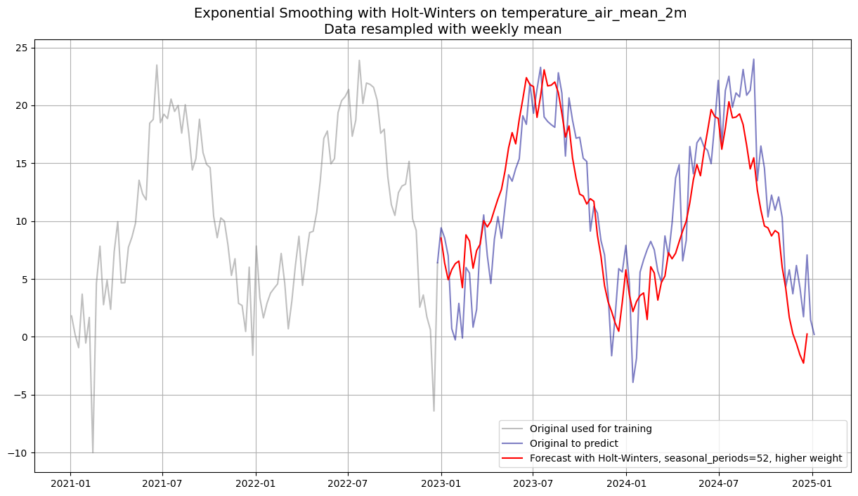

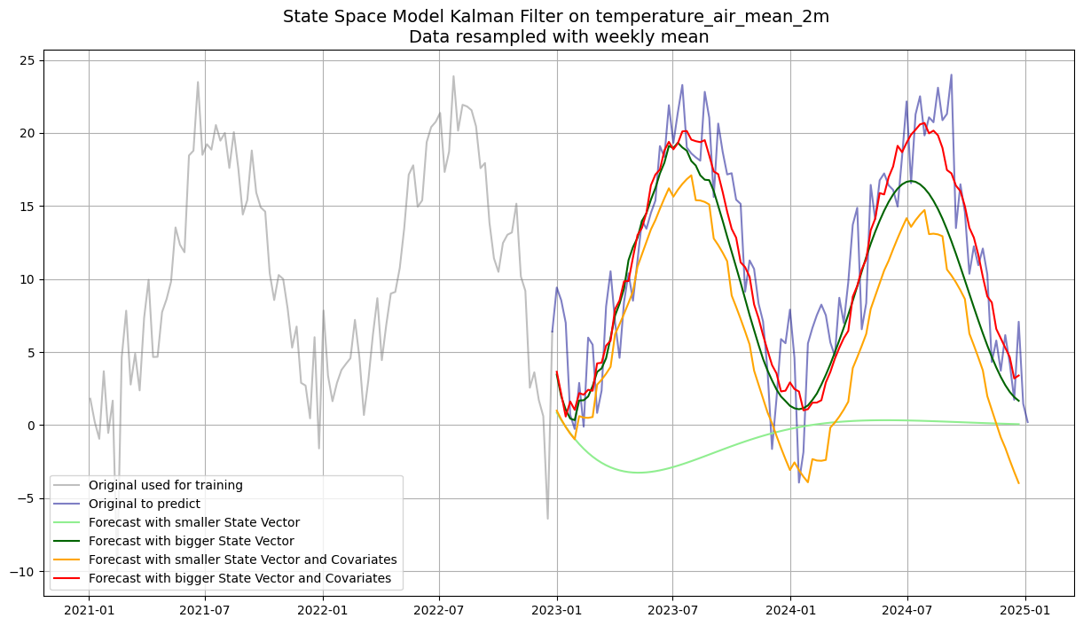
State Space Models with Kalman Filter¶

State space models represent a time series through a hidden state vector that evolves over time according to a transition equation. The Kalman filter is the optimal linear estimator of this hidden state.

Key parameter dim_x (state vector size):

Small dim_x (e.g. 2): a compact model that captures basic dynamics (level + trend-like behaviour). Less flexible but more robust on limited data.
Large dim_x (e.g. 35): can represent more complex latent structure (multiple frequency components, interactions). Prone to overfitting.

Four variants are compared: small/large state vector × with/without future covariates.

Pitfall:
The Kalman filter assumes linear, Gaussian dynamics. It will not capture non-linear patterns.
Choosing dim_x is essentially a regularisation decision. There is no closed-form rule, cross-validate on the test set.

Future Covariates - Cyclic Calendar Features¶

Covariates are additional input features that help explain the target series. Future covariates are features whose values are known in advance for the entire forecast horizon. Calendar features (month, day-of-week) are a natural choice.

Why cyclic (sin/cos) encoding for month?
A plain integer encoding (1–12) treats month 1 and month 12 as maximally distant, but they are adjacent in the calendar. Sin/cos encoding maps the month onto a circle so that the distance between consecutive months (including Dec-Jan) is uniform.

Pitfall:
Only use covariates that are genuinely available at prediction time.
Using covariates that depend on future target values (e.g. a lagged temperature from the test set) is a form of data leakage.

from darts.utils.timeseries_generation import datetime_attribute_timeseries

# Create training data as TimeSeries
temp_series_train = TimeSeries.from_series(df_w_temp_train)

# Create future covariates - month as sin / cos encoding projected 52 weeks into the future
future_cov = datetime_attribute_timeseries(temp_series_train, "month", cyclic=True, add_length=104)

future_cov.to_dataframe().loc["2020-01-01":].plot()
plt.show()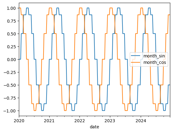


from darts.models.forecasting.kalman_forecaster import KalmanForecaster

# Fit Kalman models without covariates and predict the next 365 days
model_small = KalmanForecaster(dim_x=2)
model_small.fit(temp_series_train)
pred_small = model_small.predict(104)

model_big = KalmanForecaster(dim_x=35)
model_big.fit(temp_series_train)
pred_big = model_big.predict(104)

# Fit Kalman models with covariates and predict the next 365 days
model_small_cov = KalmanForecaster(dim_x=2)
model_small_cov.fit(temp_series_train, future_covariates=future_cov)
pred_small_cov = model_small_cov.predict(104, future_covariates=future_cov)

model_big_cov = KalmanForecaster(dim_x=35)
model_big_cov.fit(temp_series_train, future_covariates=future_cov)
pred_big_cov = model_big_cov.predict(104, future_covariates=future_cov)

plt.figure(figsize=(15, 8))
plt.plot(df_w_temp.loc["2021":"2022"], label='Original used for training', color='grey', alpha=0.5)
plt.plot(df_w_temp.loc["2022-12-25":], label='Original to predict', color='darkblue', alpha=0.5)
plt.plot(pred_small.to_series(), label=f'Forecast with smaller State Vector', color='lightgreen')
plt.plot(pred_big.to_series(), label=f'Forecast with bigger State Vector', color='darkgreen')
plt.plot(pred_small_cov.to_series(), label=f'Forecast with smaller State Vector and Covariates', color='orange')
plt.plot(pred_big_cov.to_series(), label=f'Forecast with bigger State Vector and Covariates', color='red')
plt.title(f"State Space Model Kalman Filter on {df_w_temp.name} \nData resampled with weekly mean", fontsize=14)
plt.legend()
plt.grid(True)
plt.show()