1D Harmonic Oscillator with FBPINNs#
This notebook shows you how to define your own differential equation problem and solve it using FBPINNs.
Note: The examples in this directory assume basic familiarity with PINNs. If you are new to PINNs, check out this blog post first.
Problem overview#
In this example we will use a FBPINN to solve the 1D damped harmonic oscillator:

We would like to model the displacement, \(u(t)\), of the oscillator as a function of time.
This amounts to solving the following 1D ordinary differential equation (ODE):
where \(m\) is the mass of the oscillator, \(\mu\) is the coefficient of friction and \(k\) is the spring constant.
We will focus on solving the problem in the under-damped state, i.e. where the oscillation is slowly damped by friction (as displayed in the animation above).
Mathematically, this occurs when:
Furthermore, we consider the following initial conditions of the system:
For this particular case, the exact solution is known and given by:
For a more detailed mathematical description of the harmonic oscillator, check out this blog post: https://beltoforion.de/en/harmonic_oscillator/.
How (FB)PINNs solve this problem#
PINNs use a neural network with trainable parameters \(\theta\) to directly approximate the solution to the differential equation, i.e.
Then, to learn the solution to the problem above (i.e. train the network), the following loss function is used:
The first two terms are known as the boundary loss, which try to ensure the boundary conditions are obeyed, and the last term is known as the physics loss, which minimises the residual of the differential equation throughout the problem domain. \(\{t_{i}\}_{i=1}^N\) are a set of collocation points (coordinates) sampled throughout the problem domain used to evaluate the physics loss, and \(\lambda_1\) and \(\lambda_2\) are scalar hyperparameters used to control the balence between the different terms in the loss function.
Note: FBPINNs are trained using exactly the same loss function as PINNs - the only difference is that the neural network \(N\!N(t;\theta)\) above is replaced by a summation over all subdomain networks in the FBPINN.
Workflow overview#
We will use the following steps to define and train the FBPINN:
Define the problem domain, by using the
fbpinns.domains.RectangularDomainNDclassDefine the ODE to solve, and its problem constraints, by defining our own
fbpinns.problems.ProblemclassDefine the domain decomposition used by the FBPINN, by using the
fbpinns.decompositions.RectangularDecompositionNDclassDefine the neural network placed in each subdomain, by using the
fbpinns.networks.FCNclassPass these classes and their initialisation values to a
fbpinns.constants.ConstantsobjectStart the FBPINN training by instantiating a
fbpinns.trainer.FBPINNTrainerusing theConstantsobject.
Step 1: Define problem domain#
For this example, we will use the existing fbpinns.domains.RectangularDomainND class to define the problem domain. In this case all we need to do is define the initialisation values of this class:
import numpy as np
from fbpinns.domains import RectangularDomainND

domain = RectangularDomainND
domain_init_kwargs = dict(
    xmin=np.array([0.,]),
    xmax=np.array([1.,]),# solve the problem over the domain [0, 1]
)
Step 2: Define the ODE to solve#
Next, we will define our own fbpinns.problems.Problem class to define the ODE to solve. The important things we must define in this class are:
The problem constraints: these are all the input points, any supervised labels, and the solution and gradients components required to evaluate each term (i.e. constraint) in the loss function
The loss function used to train the FBPINN, given these constraints
The exact solution, if it exists, used to test the FBPINN during training
Inheriting the Problem class#
All problem classes should inherit from the base fbpinns.problems.Problem class.
import jax.numpy as jnp
from fbpinns.problems import Problem
The base Problem class is shown below:
class Problem:
    """Base problem class to be inherited by different problem classes.

    Note all methods in this class are jit compiled / used by JAX,
    so they must not include any side-effects!
    (A side-effect is any effect of a function that doesn’t appear in its output)
    This is why only static methods are defined.
    """

    # required methods

    @staticmethod
    def init_params(*args):
        """Initialise class parameters.
        Returns tuple of dicts ({k: pytree}, {k: pytree}) containing static and trainable parameters"""

        # below parameters need to be defined
        static_params = {
            "dims":None,# (ud, xd)# dimensionality of u and x
            }
        raise NotImplementedError

    @staticmethod
    def sample_constraints(all_params, domain, key, sampler, batch_shapes):
        """Samples all constraints.
        Returns [[x_batch, *any_constraining_values, required_ujs], ...]. Each list element contains
        the x_batch points and any constraining values passed to the loss function, and the required
        solution and gradient components required in the loss function, for each constraint."""
        raise NotImplementedError

    @staticmethod
    def loss_fn(all_params, constraints):
        """Computes the PINN loss function, using constraints with the same structure output by sample_constraints"""
        raise NotImplementedError

    @staticmethod
    def exact_solution(all_params, x_batch, batch_shape=None):
        """Defines exact solution, if it exists"""
        raise NotImplementedError
A note on functional programming#
Before we explain how to implement each method, it is important to understand the semantics of the class.
fbpinnsuses JAX as its main computational engine. To be able to use JAX effectively (in particular itsjitcompilation), we need to write functionally pure code. This means that any functions we write which are compiled (which include most of the class methods above) should not have any side-effects - that is, all the input data is passed through the function parameters, all the results are output through the function results. An important consequence of this is that we should not refer to, or update, the class state (i.e. useselfin standard Python classes), as this may have unexpected consequences.
To ensure functionally purity, all the class methods above are defined as staticmethods, and any initial parameters of the class (output by init_params) are explicitly passed to each method in the all_params argument (rather than saving them to self).
Problem.init_params(*args)#
The init_params method intialises any static and trainable problem parameters.
It should return two dictionaries, one containing static parameters and the other containing trainable parameters.
For our problem, we do not want to learn any problem parameters, so the trainable parameters dictionary is empty. In the static parameters dictionary, we store all of the fixed problem parameters (namely, the values of \(\delta\) and \(\omega_0\) defined above - note, we assume \(m=1\)).
There is one extra static argument which is required - dims, which is a tuple (ud,xd) which defines the dimensionality of the solution and the problem domain (in this case, both are 1 dimensional).
@staticmethod
def init_params(d=2, w0=20):

    mu, k = 2*d, w0**2

    static_params = {
        "dims":(1,1),
        "d":d,
        "w0":w0,
        "mu":mu,
        "k":k,
        }

    return static_params, {}
Problem.sample_constraints(all_params, domain, key, sampler, batch_shapes)#
The sample_constraints method should return all the input points, any supervised labels, and the solution and gradients components required to evaluate each term (i.e. constraint) in the loss function.
It should return a constraints list where each element of the list contains the quantities required for each term in the loss function.
Defining each problem constraint#
For our problem, we have two terms (i.e. constraints) - the boundary loss and the physics loss.
For the boundary loss, we only need a single input point (\(t=0\)). We also need two supervised labels (\(u(0)=1\) and \(u_t(0)=0\)) which define the initial location and velocity of the oscillator.
We specify the input points and labels by using jnp.arrays. The input points array should have dimensionality (n,xd) where n is the number of input points and xd is the dimensionality of the input points, and any label arrays should have dimensionality (n,ld) where n is the number of input points and ld is the dimensionality of each label.
To evaluate the boundary loss, we need both the FBPINN solution (\(u\)) and its first order derivative (\(u_t\)). We specify the solution and gradients components required by using tuples, where the first value of the tuple denotes the solution component index required and its trailing tuple indicates the indices of any coordinates we require gradients with respect to (for example, (0,()) states that we need \(u\) and (0,(0,)) states that we need \(u_{t}\) for our problem).
For the physics loss, we sample input points throughout the domain (using the sample_interior helper function of the fbpinns.domains.Domain class passed to the method). We do not need any supervised labels for the physics loss, and require the FBPINN solution, and its first and second order derivatives.
Note, the number of input points for each constraint can be taken from the batch_shapes argument (fbpinns.constants.Constants.ns is passed as batch_shapes during training), and key is a jax random key.
@staticmethod
def sample_constraints(all_params, domain, key, sampler, batch_shapes):

    # physics loss
    x_batch_phys = domain.sample_interior(all_params, key, sampler, batch_shapes[0])
    required_ujs_phys = (
        (0,()),
        (0,(0,)),
        (0,(0,0))
    )

    # boundary loss
    x_batch_boundary = jnp.array([0.]).reshape((1,1))
    u_boundary = jnp.array([1.]).reshape((1,1))
    ut_boundary = jnp.array([0.]).reshape((1,1))
    required_ujs_boundary = (
        (0,()),
        (0,(0,)),
    )

    return [[x_batch_phys, required_ujs_phys], [x_batch_boundary, u_boundary, ut_boundary, required_ujs_boundary]]
loss_fn(all_params, constraints)#
The loss_fn method evaluates the FBPINN loss function, given the constraints defined by sample_constraints.
The constraints argument passed to this function has exactly the same structure as the constraints list output by sample_constraints, with two exceptions:
The
required_ujstuples are replaced withjnp.arrays containing the actual evaluated gradients of the FBPINNThe number of input points / labels (denoted by
nabove) may be smaller thannif afbpinns.schedulers.ActiveScheduleris being used.
Given this constraint list, the loss function can be easily evaluated:
@staticmethod
def loss_fn(all_params, constraints):

    mu, k = all_params["static"]["problem"]["mu"], all_params["static"]["problem"]["k"]

    # physics loss
    _, u, ut, utt = constraints[0]
    phys = jnp.mean((utt + mu*ut + k*u)**2)

    # boundary loss
    _, uc, utc, u, ut = constraints[1]
    boundary = 1e6*jnp.mean((u-uc)**2) + 1e2*jnp.mean((ut-utc)**2)

    return phys + boundary
Problem.exact_solution(all_params, x_batch, batch_shape=None)#
Finally, the exact_solution method evaluates the exact solution of the problem, if it exists, which is used to test the FBPINN during training.
The input to this function is a batch of input points (x_batch) contained in a jnp.array of shape (n, xd). The output of the function must be the solution evaluated at these points, contained in a jnp.array of shape (n, ud).
batch_shape is usually a tuple defining the underlying shape of the flattened input points (for example, during training, the input test points are always generated on a grid of shape fbpinns.constants.Constants.n_test sampling the interior of the domain and then flattened). This can be used to help compute the solution if needed.
@staticmethod
def exact_solution(all_params, x_batch, batch_shape=None):

    d, w0 = all_params["static"]["problem"]["d"], all_params["static"]["problem"]["w0"]

    w = jnp.sqrt(w0**2-d**2)
    phi = jnp.arctan(-d/w)
    A = 1/(2*jnp.cos(phi))
    cos = jnp.cos(phi + w * x_batch)
    exp = jnp.exp(-d * x_batch)
    u = exp * 2 * A * cos

    return u
The fully defined Problem class and its initial values are given below:
class HarmonicOscillator1D(Problem):
    """Solves the time-dependent damped harmonic oscillator
          d^2 u      du
        m ----- + mu -- + ku = 0
          dt^2       dt

        Boundary conditions:
        u (0) = 1
        u'(0) = 0
    """

    @staticmethod
    def init_params(d=2, w0=20):

        mu, k = 2*d, w0**2

        static_params = {
            "dims":(1,1),
            "d":d,
            "w0":w0,
            "mu":mu,
            "k":k,
            }

        return static_params, {}

    @staticmethod
    def sample_constraints(all_params, domain, key, sampler, batch_shapes):

        # physics loss
        x_batch_phys = domain.sample_interior(all_params, key, sampler, batch_shapes[0])
        required_ujs_phys = (
            (0,()),
            (0,(0,)),
            (0,(0,0))
        )

        # boundary loss
        x_batch_boundary = jnp.array([0.]).reshape((1,1))
        u_boundary = jnp.array([1.]).reshape((1,1))
        ut_boundary = jnp.array([0.]).reshape((1,1))
        required_ujs_boundary = (
            (0,()),
            (0,(0,)),
        )

        return [[x_batch_phys, required_ujs_phys], [x_batch_boundary, u_boundary, ut_boundary, required_ujs_boundary]]

    @staticmethod
    def loss_fn(all_params, constraints):

        mu, k = all_params["static"]["problem"]["mu"], all_params["static"]["problem"]["k"]

        # physics loss
        _, u, ut, utt = constraints[0]
        phys = jnp.mean((utt + mu*ut + k*u)**2)

        # boundary loss
        _, uc, utc, u, ut = constraints[1]
        boundary = 1e6*jnp.mean((u-uc)**2) + 1e2*jnp.mean((ut-utc)**2)

        return phys + boundary

    @staticmethod
    def exact_solution(all_params, x_batch, batch_shape=None):

        d, w0 = all_params["static"]["problem"]["d"], all_params["static"]["problem"]["w0"]

        w = jnp.sqrt(w0**2-d**2)
        phi = jnp.arctan(-d/w)
        A = 1/(2*jnp.cos(phi))
        cos = jnp.cos(phi + w * x_batch)
        exp = jnp.exp(-d * x_batch)
        u = exp * 2 * A * cos

        return u

problem = HarmonicOscillator1D
problem_init_kwargs=dict(
    d=2, w0=80,# define the ODE parameters
)
Step 3: Define the domain decomposition used by the FBPINN#
Next, we use the existing fbpinns.decompositions.RectangularDecompositionND class to define the domain decomposition used by the FBPINN. In this case all we need to do is define the initialisation values of this class:
from fbpinns.decompositions import RectangularDecompositionND

decomposition = RectangularDecompositionND# use a rectangular domain decomposition
decomposition_init_kwargs=dict(
    subdomain_xs=[np.linspace(0,1,15)],# use 15 equally spaced subdomains
    subdomain_ws=[0.15*np.ones((15,))],# with widths of 0.15
    unnorm=(0.,1.),# define unnormalisation of the subdomain networks
)
Step 4: Define the neural network placed in each subdomain#
Next, we use the existing fbpinns.networks.FCN class to define the neural network placed in each subdomain. In this case all we need to do is define the initialisation values of this class:
from fbpinns.networks import FCN

network = FCN# place a fully-connected network in each subdomain
network_init_kwargs=dict(
    layer_sizes=[1,32,1],# with 2 hidden layers
)
Step 5: Create a Constants object#
Now that we have defined our Domain, Problem, Decomposition and Network and their initialisation values, we use these to instantiate a fbpinns.constants.Constants object (other training hyperparameters can be passed to the Constants object as necessary):
from fbpinns.constants import Constants

c = Constants(
    domain=domain,
    domain_init_kwargs=domain_init_kwargs,
    problem=problem,
    problem_init_kwargs=problem_init_kwargs,
    decomposition=decomposition,
    decomposition_init_kwargs=decomposition_init_kwargs,
    network=network,
    network_init_kwargs=network_init_kwargs,
    ns=((200,),),# use 200 collocation points for training
    n_test=(500,),# use 500 points for testing
    n_steps=20000,# number of training steps
    clear_output=True,
)

print(c)
<fbpinns.constants.Constants object at 0x135df33d0>
run: test
domain: <class 'fbpinns.domains.RectangularDomainND'>
domain_init_kwargs: {'xmin': array([0.]), 'xmax': array([1.])}
problem: <class '__main__.HarmonicOscillator1D'>
problem_init_kwargs: {'d': 2, 'w0': 80}
decomposition: <class 'fbpinns.decompositions.RectangularDecompositionND'>
decomposition_init_kwargs: {'subdomain_xs': [array([0.        , 0.07142857, 0.14285714, 0.21428571, 0.28571429,
       0.35714286, 0.42857143, 0.5       , 0.57142857, 0.64285714,
       0.71428571, 0.78571429, 0.85714286, 0.92857143, 1.        ])], 'subdomain_ws': [array([0.15, 0.15, 0.15, 0.15, 0.15, 0.15, 0.15, 0.15, 0.15, 0.15, 0.15,
       0.15, 0.15, 0.15, 0.15])], 'unnorm': (0.0, 1.0)}
network: <class 'fbpinns.networks.FCN'>
network_init_kwargs: {'layer_sizes': [1, 32, 1]}
n_steps: 20000
scheduler: <class 'fbpinns.schedulers.AllActiveSchedulerND'>
scheduler_kwargs: {}
ns: ((200,),)
n_test: (500,)
sampler: grid
optimiser: <function adam at 0x136170430>
optimiser_kwargs: {'learning_rate': 0.001}
seed: 0
summary_freq: 1000
test_freq: 1000
model_save_freq: 10000
show_figures: True
save_figures: False
clear_output: True
hostname: pickwick-iii.local
Step 6: Train the FBPINN using a FBPINNTrainer#
Finally, we can train the FBPINN by using a fbpinns.trainers.FBPINNTrainer:
from fbpinns.trainers import FBPINNTrainer

run = FBPINNTrainer(c)
all_params = run.train()
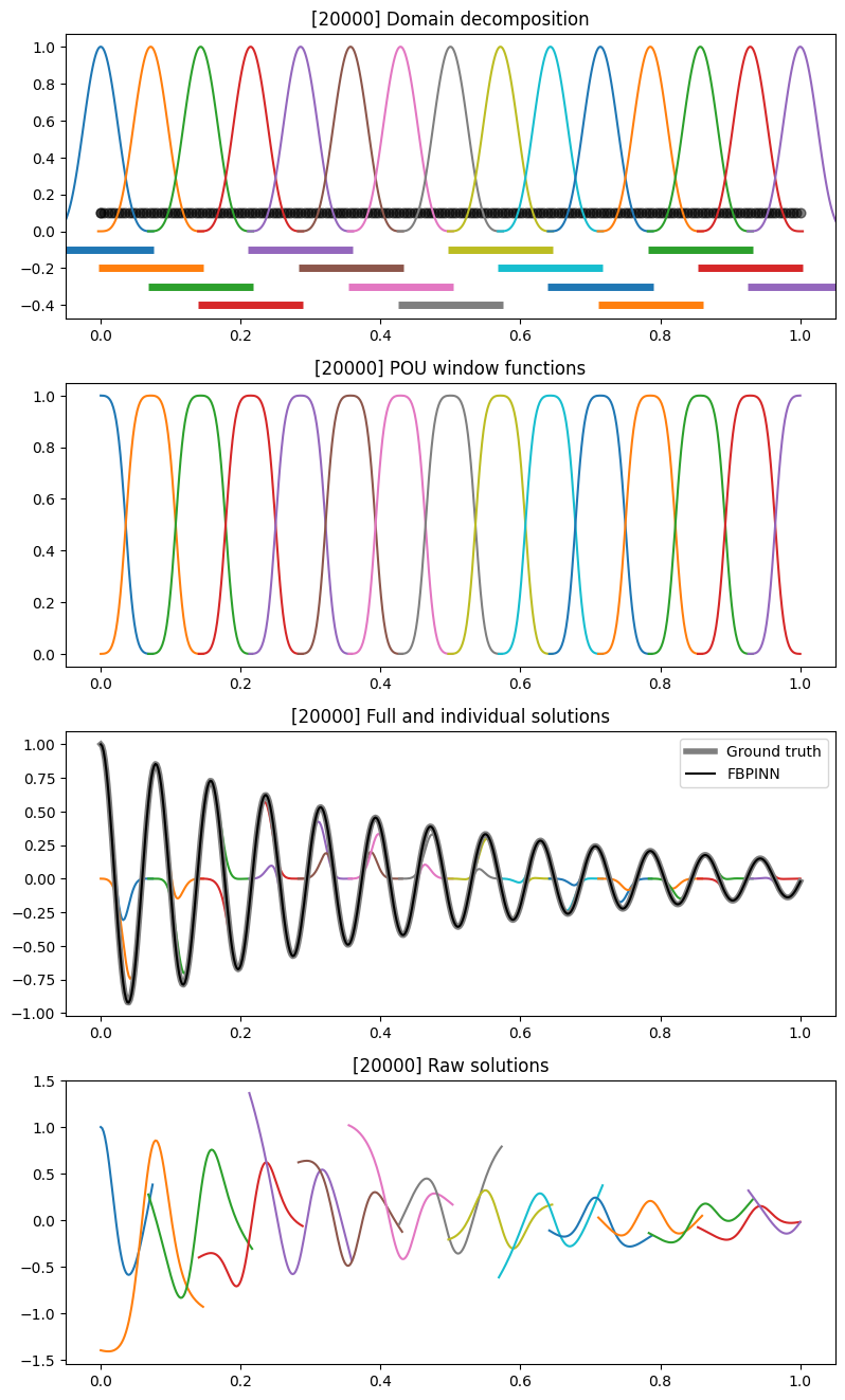
[INFO] 2025-05-05 13:03:43 - [i: 20000/20000] Training complete