🚀 Access curated PNW Dataset with SeisBench APIs#

Author: Yiyu Ni
Goal: This notebook demonstrates how to access the curated PNW seismic dataset with SeisBench APIs.
import torch
import numpy as np
import pandas as pd
import matplotlib.pyplot as plt
import seisbench.data as sbd
import seisbench.generate as sbg
1. Load the dataset#
A dataset is made by the waveform file (in hdf5 format, sometime also called h5) and the perspective metadata file (in csv format). See the structure in the /data/horse/ws/s4122485-ai4seismology/data/earthquake_seismology folder with two small datasets (i.e., mesoPNW).
🚀 Read more about SeisBench data format: https://seisbench.readthedocs.io/en/stable/pages/data_format.html
Download from Google Drive stored data.
# !pip install gdown
# import os
# import sys
# import subprocess
# import gdown


# # Create the directory structure if it doesn't exist
# dataset_name = "downloadedPNW"  # Name for the new dataset directory
# dataset_dir = os.path.join("./pnwml", dataset_name)
# os.makedirs(dataset_dir, exist_ok=True)

# # Download the dataset from Google Drive
# url = "https://drive.google.com/file/d/1SrbiQpBpU6mPq5Un_lJpPcfBekwczLzp/view?usp=share_link"
# output = os.path.join(dataset_dir, "waveforms.hdf5")


# url2="https://drive.google.com/file/d/1HK2AuWPQj3dCdKShYcJ7a5E577XASrab/view?usp=share_link"
# output2 = os.path.join(dataset_dir, "metadata.csv")
# # Use gdown to download from Google Drive
# print(f"Downloading dataset from Google Drive to {output}...")
# gdown.download(url, output, quiet=False, fuzzy=True)
# print(f"Downloading dataset from Google Drive to {output2}...")
# gdown.download(url, output2, quiet=False, fuzzy=True)

# print(f"Dataset downloaded successfully to {dataset_dir}!")
We pre-downloaded the data, so please now copy it to your local folder
os.mkdir("../data/pnwml", exist_ok=True)
!cp /data/horse/ws/s4122485-ai4seismology/data/earthquake_seismology/*hdf5 ../data/pnwml
!cp /data/horse/ws/s4122485-ai4seismology/data/earthquake_seismology/*csv ../data/pnwml
The metadata.csv represents a table of metadata for each data sample. It also documents where to locate the waveform. We will have a better view of this table later.
! head -n 5 ../data/pnwml/mesoPNW/metadata.csv
event_id,source_origin_time,source_latitude_deg,source_longitude_deg,source_type,source_depth_km,preferred_source_magnitude,preferred_source_magnitude_type,preferred_source_magnitude_uncertainty,source_depth_uncertainty_km,source_horizontal_uncertainty_km,station_network_code,station_channel_code,station_code,station_location_code,station_latitude_deg,station_longitude_deg,station_elevation_m,trace_name,trace_sampling_rate_hz,trace_start_time,trace_S_arrival_sample,trace_P_arrival_sample,trace_S_arrival_uncertainty_s,trace_P_arrival_uncertainty_s,trace_P_polarity,trace_S_onset,trace_P_onset,trace_snr_db,source_type_pnsn_label,source_local_magnitude,source_local_magnitude_uncertainty,source_duration_magnitude,source_duration_magnitude_uncertainty,source_hand_magnitude,trace_missing_channel,trace_has_offset,bucket,tindex
uw10564613,2002-10-03T01:56:49.530000Z,48.553,-122.52,earthquake,14.907,2.1,md,0.03,1.68,0.694,UW,BH,GNW,--,47.564,-122.825,220.0,"bucket4$0,:3,:15001",100,2002-10-03T01:55:59.530000Z,8097,6733,0.04,0.02,undecidable,,,6.135|3.065|11.766,eq,,,2.1,0.03,,0,1,4,0
uw10564613,2002-10-03T01:56:49.530000Z,48.553,-122.52,earthquake,14.907,2.1,md,0.03,1.68,0.694,UW,EH,RPW,--,48.448,-121.515,850.0,"bucket9$0,:3,:15001",100,2002-10-03T01:55:59.530000Z,7258,6238,0.04,0.01,undecidable,,,nan|nan|22.583,eq,,,2.1,0.03,,2,0,9,0
uw10564613,2002-10-03T01:56:49.530000Z,48.553,-122.52,earthquake,14.907,2.1,md,0.03,1.68,0.694,UW,BH,SQM,--,48.074,-123.048,45.0,"bucket4$1,:3,:15001",100,2002-10-03T01:55:59.530000Z,7037,6113,0.08,0.04,undecidable,,,1.756|3.057|3.551,eq,,,2.1,0.03,,0,1,4,1
uw10564613,2002-10-03T01:56:49.530000Z,48.553,-122.52,earthquake,14.907,2.1,md,0.03,1.68,0.694,UW,EH,MCW,--,48.679,-122.833,693.0,"bucket7$0,:3,:15001",100,2002-10-03T01:55:59.530000Z,5894,5442,0.04,0.01,negative,,,nan|nan|27.185,eq,,,2.1,0.03,,2,0,7,0
We can load the dataset using seisbench.data as a WaveformDataset class.
dataset = sbd.WaveformDataset("../data/pnwml/mesoPNW/")

print(f"The dataset contains {len(dataset)} samples.")
2025-04-23 21:41:11,945 | seisbench | WARNING | Dimension order not specified in data set. Assuming CW.
The dataset contains 18640 samples.
The metadata can be accessed by the .metadata attribute of the dataset as a pd.DataFrame object.
pd.set_option('display.max_columns', None) # show all columns
meta = dataset.metadata
meta.head()
| index | event_id | source_origin_time | source_latitude_deg | source_longitude_deg | source_type | source_depth_km | preferred_source_magnitude | preferred_source_magnitude_type | preferred_source_magnitude_uncertainty | source_depth_uncertainty_km | source_horizontal_uncertainty_km | station_network_code | station_channel_code | station_code | station_location_code | station_latitude_deg | station_longitude_deg | station_elevation_m | trace_name | trace_sampling_rate_hz | trace_start_time | trace_S_arrival_sample | trace_P_arrival_sample | trace_S_arrival_uncertainty_s | trace_P_arrival_uncertainty_s | trace_P_polarity | trace_S_onset | trace_P_onset | trace_snr_db | source_type_pnsn_label | source_local_magnitude | source_local_magnitude_uncertainty | source_duration_magnitude | source_duration_magnitude_uncertainty | source_hand_magnitude | trace_missing_channel | trace_has_offset | bucket | tindex | trace_chunk | trace_component_order | |
|---|---|---|---|---|---|---|---|---|---|---|---|---|---|---|---|---|---|---|---|---|---|---|---|---|---|---|---|---|---|---|---|---|---|---|---|---|---|---|---|---|---|---|
| 0 | 0 | uw10564613 | 2002-10-03T01:56:49.530000Z | 48.553 | -122.520 | earthquake | 14.907 | 2.1 | md | 0.03 | 1.68 | 0.694 | UW | BH | GNW | -- | 47.564 | -122.825 | 220.0 | bucket4$0,:3,:15001 | 100.0 | 2002-10-03T01:55:59.530000Z | 8097 | 6733 | 0.04 | 0.02 | undecidable | NaN | NaN | 6.135|3.065|11.766 | eq | NaN | NaN | 2.1 | 0.03 | NaN | 0 | 1 | 4 | 0 | ENZ | |
| 1 | 1 | uw10564613 | 2002-10-03T01:56:49.530000Z | 48.553 | -122.520 | earthquake | 14.907 | 2.1 | md | 0.03 | 1.68 | 0.694 | UW | EH | RPW | -- | 48.448 | -121.515 | 850.0 | bucket9$0,:3,:15001 | 100.0 | 2002-10-03T01:55:59.530000Z | 7258 | 6238 | 0.04 | 0.01 | undecidable | NaN | NaN | nan|nan|22.583 | eq | NaN | NaN | 2.1 | 0.03 | NaN | 2 | 0 | 9 | 0 | ENZ | |
| 2 | 2 | uw10564613 | 2002-10-03T01:56:49.530000Z | 48.553 | -122.520 | earthquake | 14.907 | 2.1 | md | 0.03 | 1.68 | 0.694 | UW | BH | SQM | -- | 48.074 | -123.048 | 45.0 | bucket4$1,:3,:15001 | 100.0 | 2002-10-03T01:55:59.530000Z | 7037 | 6113 | 0.08 | 0.04 | undecidable | NaN | NaN | 1.756|3.057|3.551 | eq | NaN | NaN | 2.1 | 0.03 | NaN | 0 | 1 | 4 | 1 | ENZ | |
| 3 | 3 | uw10564613 | 2002-10-03T01:56:49.530000Z | 48.553 | -122.520 | earthquake | 14.907 | 2.1 | md | 0.03 | 1.68 | 0.694 | UW | EH | MCW | -- | 48.679 | -122.833 | 693.0 | bucket7$0,:3,:15001 | 100.0 | 2002-10-03T01:55:59.530000Z | 5894 | 5442 | 0.04 | 0.01 | negative | NaN | NaN | nan|nan|27.185 | eq | NaN | NaN | 2.1 | 0.03 | NaN | 2 | 0 | 7 | 0 | ENZ | |
| 4 | 4 | uw10568748 | 2002-09-26T07:00:04.860000Z | 48.481 | -123.133 | earthquake | 22.748 | 2.9 | md | 0.03 | 0.91 | 0.672 | UW | HH | SP2 | -- | 47.556 | -122.249 | 30.0 | bucket3$0,:3,:15001 | 100.0 | 2002-09-26T06:59:14.860000Z | 8647 | 6948 | 0.04 | 0.01 | negative | NaN | NaN | 10.881|17.107|2.242 | eq | NaN | NaN | 2.9 | 0.03 | NaN | 0 | 1 | 3 | 0 | ENZ |
2. SeisBench APIs for data access and augmentataion#
A generator is employed as a dataset wrapper, where users specify APIs for data pre-processing and augmentation.
🚀 See https://seisbench.readthedocs.io/en/latest/pages/documentation/generate.html for all supported augmentation methods.
generator = sbg.GenericGenerator(dataset)

phase_dict = {"trace_P_arrival_sample": "P",
              "trace_S_arrival_sample": "S"}

augmentations = [
    sbg.WindowAroundSample(list(phase_dict.keys()),
                           samples_before=5000,
                           windowlen=10000,
                           selection="first",
                           strategy="pad"),
    sbg.RandomWindow(windowlen=6000),
    sbg.Normalize(demean_axis=-1,
                  amp_norm_axis=-1,
                  amp_norm_type="peak"),
    sbg.ChangeDtype(np.float32),
    sbg.DetectionLabeller("trace_P_arrival_sample",
                          "trace_S_arrival_sample",
                          factor=1.,
                          dim=0,
                          key=('X', 'y2')),
    sbg.ProbabilisticLabeller(label_columns=phase_dict,
                              shape='triangle',
                              sigma=10,
                              dim=0,
                              key=('X', 'y1'))
]
generator.add_augmentations(augmentations)
print(generator)
<class 'seisbench.generate.generator.GenericGenerator'> with 6 augmentations:
 1.	WindowAroundSample (metadata_keys=['trace_P_arrival_sample', 'trace_S_arrival_sample'], samples_before=5000, selection=first)
 2.	RandomWindow (low=None, high=None)
 3.	Normalize (Demean (axis=-1), Amplitude normalization (type=peak, axis=-1))
 4.	ChangeDtype (dtype=<class 'numpy.float32'>, key=('X', 'X'))
 5.	DetectionLabeller (label_type=multi_class, dim=0)
 6.	ProbabilisticLabeller (label_type=multi_class, dim=0)
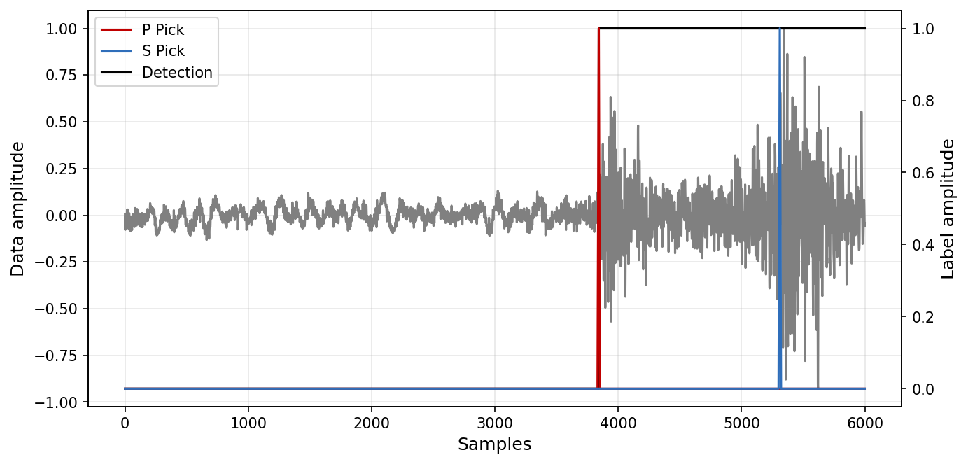
A generator is indexable. You can use an index to access a specific data sample, and plot the waveforms.
idx = 101
sp = generator[idx]
for k, v in sp.items():
    print({k: v})
    print({k: v.shape})
    print("===============")
{'X': array([[ 0.00743013, -0.056532  , -0.07826877, ..., -0.02479234,
        -0.05956911, -0.0431165 ],
       [-0.03419543, -0.03570489, -0.02515121, ...,  0.02853432,
         0.01560807, -0.00841141],
       [ 0.05039116,  0.0543057 ,  0.05657212, ...,  0.06317093,
         0.0874832 ,  0.08027197]], dtype=float32)}
{'X': (3, 6000)}
===============
{'y2': array([[0., 0., 0., ..., 1., 1., 1.]])}
{'y2': (1, 6000)}
===============
{'y1': array([[0., 0., 0., ..., 0., 0., 0.],
       [0., 0., 0., ..., 0., 0., 0.],
       [1., 1., 1., ..., 1., 1., 1.]])}
{'y1': (3, 6000)}
===============
plt.figure(figsize = (10, 5), dpi = 150)
plt.plot(sp['X'][0, :].T, c='gray')
plt.xlabel("Samples", fontsize = 12)
plt.ylabel("Data amplitude", fontsize = 12)
plt.grid(True, alpha=0.3)

ax = plt.gca().twinx()
ax.plot(sp['y1'][0, :].T, label = "P Pick", c="#c00000")
ax.plot(sp['y1'][1, :].T, label = "S Pick", c="#2f6eba")
ax.plot(sp['y2'][0, :].T, label = "Detection", color='k', zorder=-1)
plt.ylabel("Label amplitude", fontsize = 12)

plt.legend(loc = 'upper left')
<matplotlib.legend.Legend at 0x28c1acf70>
3. Loading data in batch#
Machine Learning model training usually load data in batch. The generator object can be wrapped by the pytorch API torch.utils.data.DataLoader to generate samples in batch. See examples below that creates a data loader and return 256 samples in batch.
batch_size = 256
loader = torch.utils.data.DataLoader(generator,
                    batch_size=batch_size, shuffle=True, num_workers=0)
See the changes in the array sizez as well as the array type.
for i in loader:
    for k, v in i.items():
        print({k: v})
        print({k: v.shape})
        print("===============")
    break
{'X': tensor([[[-0.3553, -0.3545, -0.3528,  ..., -0.1436, -0.1028, -0.0371],
         [ 0.1409,  0.1364,  0.1332,  ..., -0.0967, -0.0943, -0.0863],
         [-0.1704, -0.1658, -0.1625,  ...,  0.3062,  0.3093,  0.3049]],

        [[-0.1790, -0.1660, -0.1899,  ...,  0.1565, -0.0152, -0.1217],
         [ 0.0000,  0.0000,  0.0000,  ...,  0.0000,  0.0000,  0.0000],
         [ 0.0000,  0.0000,  0.0000,  ...,  0.0000,  0.0000,  0.0000]],

        [[-0.0510, -0.0510, -0.0304,  ...,  0.0722,  0.1003,  0.0997],
         [ 0.0000,  0.0000,  0.0000,  ...,  0.0000,  0.0000,  0.0000],
         [ 0.0000,  0.0000,  0.0000,  ...,  0.0000,  0.0000,  0.0000]],

        ...,

        [[ 0.0411,  0.0343,  0.0308,  ...,  0.1134,  0.1103,  0.1096],
         [-0.0015, -0.0034, -0.0053,  ...,  0.0106,  0.0076,  0.0048],
         [-0.0312, -0.0308, -0.0346,  ...,  0.0256,  0.0235,  0.0219]],

        [[ 0.0196, -0.0742, -0.0818,  ..., -0.0292,  0.0280,  0.0524],
         [ 0.0552,  0.0740,  0.0378,  ...,  0.0497,  0.0277, -0.0029],
         [-0.0106, -0.0176, -0.0112,  ...,  0.0353,  0.0058, -0.0474]],

        [[-0.0100, -0.0098,  0.0043,  ..., -0.0214, -0.0343, -0.0205],
         [ 0.0000,  0.0000,  0.0000,  ...,  0.0000,  0.0000,  0.0000],
         [ 0.0000,  0.0000,  0.0000,  ...,  0.0000,  0.0000,  0.0000]]])}
{'X': torch.Size([256, 3, 6000])}
===============
{'y2': tensor([[[0., 0., 0.,  ..., 0., 0., 0.]],

        [[0., 0., 0.,  ..., 0., 0., 0.]],

        [[0., 0., 0.,  ..., 0., 0., 0.]],

        ...,

        [[0., 0., 0.,  ..., 0., 0., 0.]],

        [[0., 0., 0.,  ..., 0., 0., 0.]],

        [[0., 0., 0.,  ..., 0., 0., 0.]]], dtype=torch.float64)}
{'y2': torch.Size([256, 1, 6000])}
===============
{'y1': tensor([[[0., 0., 0.,  ..., 0., 0., 0.],
         [0., 0., 0.,  ..., 0., 0., 0.],
         [1., 1., 1.,  ..., 1., 1., 1.]],

        [[0., 0., 0.,  ..., 0., 0., 0.],
         [0., 0., 0.,  ..., 0., 0., 0.],
         [1., 1., 1.,  ..., 1., 1., 1.]],

        [[0., 0., 0.,  ..., 0., 0., 0.],
         [0., 0., 0.,  ..., 0., 0., 0.],
         [1., 1., 1.,  ..., 1., 1., 1.]],

        ...,

        [[0., 0., 0.,  ..., 0., 0., 0.],
         [0., 0., 0.,  ..., 0., 0., 0.],
         [1., 1., 1.,  ..., 1., 1., 1.]],

        [[0., 0., 0.,  ..., 0., 0., 0.],
         [0., 0., 0.,  ..., 0., 0., 0.],
         [1., 1., 1.,  ..., 1., 1., 1.]],

        [[0., 0., 0.,  ..., 0., 0., 0.],
         [0., 0., 0.,  ..., 0., 0., 0.],
         [1., 1., 1.,  ..., 1., 1., 1.]]], dtype=torch.float64)}
{'y1': torch.Size([256, 3, 6000])}
===============
Reference#
Ni, Y., Hutko, A., Skene, F., Denolle, M., Malone, S., Bodin, P., Hartog, R., & Wright, A. (2023). Curated Pacific Northwest AI-ready Seismic Dataset. Seismica, 2(1). https://doi.org/10.26443/seismica.v2i1.368
Woollam, J., Münchmeyer, J., Tilmann, F., Rietbrock, A., Lange, D., Bornstein, T., … & Soto, H. (2022). SeisBench—A toolbox for machine learning in seismology. Seismological Society of America, 93(3), 1695-1709.