Data Transformation

This notebook focuses on transforming cleaned data into analysis-ready features.

import pandas as pd
import matplotlib.pyplot as plt
import seaborn as sns
from sklearn.preprocessing import MinMaxScaler, StandardScaler

patients_cleaned = pd.read_csv("data/patients_cleaned.csv")

patients_cleaned.head()

	patient_id	age	admission_date	discharge_date	gender	weight	height	blood_pressure	admission_unit	albumin_g_dl
0	1	39.0	2023-01-05	2023-01-10	f	78.0	184.0	130.0	Surgery	1.00
1	2	60.0	2023-02-11	2023-02-20	m	55.0	180.0	90.0	Cardiol.	4.26
2	4	50.0	2023-03-20	2023-03-25	f	70.0	179.0	110.0	Intensive Care U.	3.10
3	10	45.0	2023-07-05	2023-07-15	m	90.0	165.0	80.0	Neurology	3.10
4	12	90.0	2023-08-10	2023-08-20	female	45.0	170.0	60.0	Intensive Care U.	4.26

#patients_cleaned.info()

1 Checking categorical variables

• Categorical variables often contain multiple spellings or encodings for the same concept. We need to standardize these.

• Here we focus on the gender column:

  • First, we inspect unique values and their counts.

  • Then we replace inconsistent entries with a standard value.

• Casting to category dtype can reduce memory and make intent explicit.

# Show number of unique categories and their counts
patients_cleaned['gender'].value_counts(dropna=False)

gender
m         9
male      9
f         6
female    2
Name: count, dtype: int64

# Correct inconsistent entries - f -> female, m -> male
patients_cleaned['gender'] = patients_cleaned['gender'].replace('f', 'female')
patients_cleaned['gender'] = patients_cleaned['gender'].replace('m', 'male')

patients_cleaned['gender'].value_counts(dropna=False)

gender
male      18
female     8
Name: count, dtype: int64

# visualize gender distribution

Check admission_unit for unique values

# Check unique values in admission_unit
patients_cleaned['admission_unit'].value_counts(dropna=False)

admission_unit
Intensive Care U.    5
Psychiatry           5
Cardiol.             3
Surgery              2
Neurology            2
Orthopedics          2
Pediatrics           2
Emergency Room       2
General Medicine     2
Oncology             1
Name: count, dtype: int64

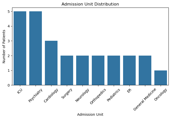
Rename inconsistent entries

# Standardize admission_unit entries
patients_cleaned['admission_unit'] = patients_cleaned['admission_unit'].replace({'Emergency Room': 'ER', 'Intensive Care U.': 'ICU', 'Cardiol.': 'Cardiology'})

# visualize admission_unit distribution

plt.figure(figsize=(8,4))
sns.countplot(data=patients_cleaned, x='admission_unit', order=patients_cleaned['admission_unit'].value_counts().index)
plt.title('Admission Unit Distribution')
plt.ylabel('Number of Patients')
plt.xlabel('Admission Unit')
plt.xticks(rotation=45)
plt.show()

2 Encoding categorical variables for modeling

• Many models require numeric inputs. pd.get_dummies() creates one-hot encoded columns for categorical variables.

• For high-cardinality categorical features you may want alternative encoding strategies (target encoding, embedding, hashing).

One-hot encoding for ‘gender’

# One-hot encode gender
patients_cleaned = pd.get_dummies(patients_cleaned, columns=['gender'], drop_first=True)

Label Encoding for ‘admission_unit’

• For admission_unit with multiple categories, we use label encoding to convert categories to integer codes.

• This is simple but imposes an ordinal relationship. For non-ordinal categories, one-hot encoding is often preferred.

• Here we demonstrate label encoding for variety.

• First convert to ‘category’ dtype, then use .cat.codes to get integer codes.

• Note: In practice, use sklearn’s LabelEncoder or OrdinalEncoder for more control.

# Convert admission_unit to 'category' dtype
patients_cleaned['admission_unit_encoded'] = patients_cleaned['admission_unit'].astype('category')

# Label encode admission_unit
patients_cleaned['admission_unit_encoded'] = patients_cleaned['admission_unit_encoded'].cat.codes

patients_cleaned.head()

	patient_id	age	admission_date	discharge_date	weight	height	blood_pressure	admission_unit	albumin_g_dl	gender_male	admission_unit_encoded
0	1	39.0	2023-01-05	2023-01-10	78.0	184.0	130.0	Surgery	1.00	False	9
1	2	60.0	2023-02-11	2023-02-20	55.0	180.0	90.0	Cardiology	4.26	True	0
2	4	50.0	2023-03-20	2023-03-25	70.0	179.0	110.0	ICU	3.10	False	3
3	10	45.0	2023-07-05	2023-07-15	90.0	165.0	80.0	Neurology	3.10	True	4
4	12	90.0	2023-08-10	2023-08-20	45.0	170.0	60.0	ICU	4.26	False	3

3 Feature engineering - creating new features from existing ones

• BMI (Body Mass Index) is a common clinical feature derived from weight and height.

• BMI = weight (kg) / (height (m))2

• In our dataset height is in cm, so it needs to be converted before calculation.

# Compute BMI (height in cm -> convert to meters)
patients_cleaned['BMI'] = patients_cleaned['weight'] / (patients_cleaned['height']/100)**2

# Inspect BMI distribution and missingness
patients_cleaned['BMI'].describe()

count    26.000000
mean     25.087716
std       6.945768
min      14.527376
25%      21.232993
50%      22.505044
75%      29.602852
max      40.562466
Name: BMI, dtype: float64

Save transformed data

# Save the transformed dataset
patients_cleaned.to_csv("data/patients_transformed.csv", index=False)

4 Scaling and standardization

• Many ML algorithms assume features are on similar scales

• MinMaxScaler rescales to [0,1]

• StandardScaler centers to mean=0 and std=1

We demonstrate both for different use cases.

Method 1: Min-Max Scaling

# Demonstrate MinMax scaling for 'age' and Standard scaling for blood pressure
minmax = MinMaxScaler()
patients_cleaned['age_minmax'] = minmax.fit_transform(patients_cleaned[['age']])

Method 2: Standardization

std = StandardScaler()
patients_cleaned['bp_std'] = std.fit_transform(patients_cleaned[['blood_pressure']])

patients_cleaned.head()

	patient_id	age	admission_date	discharge_date	weight	height	blood_pressure	admission_unit	albumin_g_dl	gender_male	admission_unit_encoded	BMI	age_minmax	bp_std
0	1	39.0	2023-01-05	2023-01-10	78.0	184.0	130.0	Surgery	1.00	False	9	23.038752	0.105263	1.274066
1	2	60.0	2023-02-11	2023-02-20	55.0	180.0	90.0	Cardiology	4.26	True	0	16.975309	0.473684	-0.436090
2	4	50.0	2023-03-20	2023-03-25	70.0	179.0	110.0	ICU	3.10	False	3	21.847009	0.298246	0.418988
3	10	45.0	2023-07-05	2023-07-15	90.0	165.0	80.0	Neurology	3.10	True	4	33.057851	0.210526	-0.863629
4	12	90.0	2023-08-10	2023-08-20	45.0	170.0	60.0	ICU	4.26	False	3	15.570934	1.000000	-1.718707

Further preprocessing for modeling

• scaling all numeric features

• dropping any remaining irrelevant columns

• handling any remaining missing values

• drop identifier patient_id

Exercise — Data Transformation

1. Standardize the blood_pressure column (use StandardScaler - is already imported), store as bp_standardized.

2. Create a new feature length_of_stay as the difference in days between discharge_date and admission_date. (Hint: columns need to be datetime dtype)

3. Plot a histogram of the computed BMI.

# 1. Standardize blood_pressure

# 2. Create length_of_stay feature

# 3. Plot histogram of BMI