Inspecting 3D image data with pyclesperanto

This notebook demonstrates how to navigate through 3D images.

import numpy as np
import matplotlib
import matplotlib.pyplot as plt
from skimage.io import imread
import stackview

# Laod example data
input_image = imread('data/Haase_MRT_tfl3d1.tif')

This image is an image stack which can be quickly visualized like this:

stackview.animate(input_image[::5,::2,::2])

Using the stackview.insight method we can quickly read image shape and intensity range. It also gives us a view of the entire dataset, an intensity projection actually.

stackview.insight(input_image)

shape (192, 256, 256) dtype uint8 size 12.0 MB min 0 max 255

Selecting slices

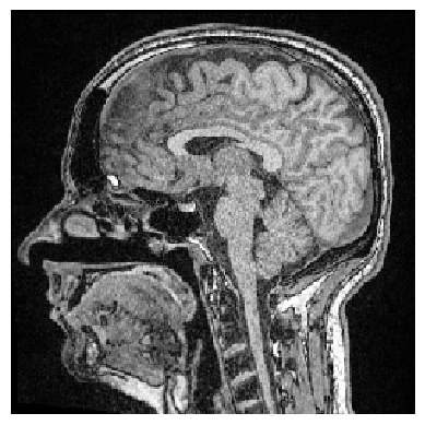
In order to visualize specific slices, we can select them.

image_slice = input_image[100]

# show result
stackview.imshow(image_slice)

We can also do this interactively.

stackview.slice(input_image)

Intensity projections

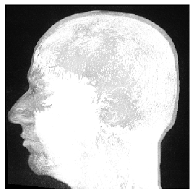
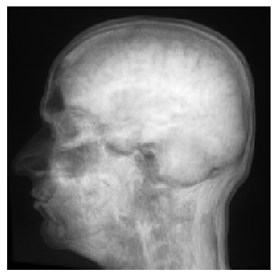
In order to take a look at the entire stack, we can do projections.

projection_max = input_image.max(axis=0)

stackview.imshow(projection_max)

projection_mean = input_image.mean(axis=0)

stackview.imshow(projection_mean)

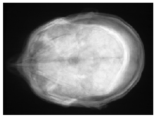
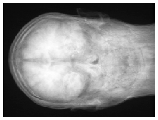
We can also do this in different directions

projection_mean = input_image.mean(axis=1)

stackview.imshow(projection_mean)

projection_mean = input_image.mean(axis=2)

stackview.imshow(projection_mean)

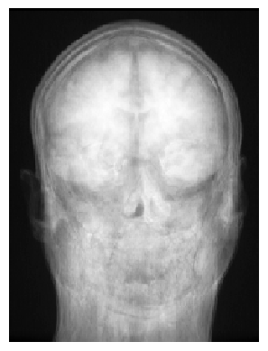
And we can transpose the image axes in case that’s necessary.

projection_mean = input_image.mean(axis=2).T

stackview.imshow(projection_mean)

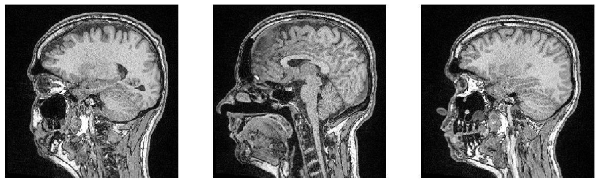
Subplots can help us to get an overview of the dataset

fig, axs = plt.subplots(1, 3, figsize=(15, 7))
stackview.imshow(input_image[75], plot=axs[0])
stackview.imshow(input_image[100], plot=axs[1])
stackview.imshow(input_image[125], plot=axs[2])

Exercise

Crop out Robert’s nose programmatically. Hint: Use stackview.crop to navigate the dataset.

stackview.crop(input_image)