Simulation of image formation + image restoration

In this notebook we artifically assemble a microscope image from simlulated nuclei, noise and background. Afterwards, we use classical image processing techniques to remove noise and background.

import pyclesperanto as cle
import numpy as np

image_size = (100, 100)

# noise configuration
noise_level = 2

# background configuration
camera_offset = 100
background_sigma = 25
background_intensity = 5

# nuclei configuration
nuclei_radius = 5
nuclei_blur_sigma = 1
nuclei_number = 10
nuclei_intensity = 5

# by pinning the random seed, we can make the code repeatable
np.random.seed(42)

Noise

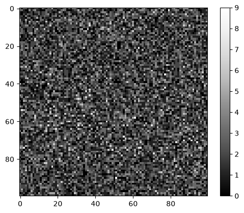
Here we assume that the noise in the image is Poisson distributed, a common assumtion in microscopy.

noise_image = np.random.poisson(noise_level, image_size)

cle.imshow(noise_image, colorbar=True)

Background

Background intensity in fluorescence microscopy images typically comes from out-of-focus light. We can simulate this by placing light sources as single pixels and blurring them with a Gaussian filter. Furthermore, many microscope cameras have a so called camera offset. No pixel will ever have intensity below this value.

# create empty image
background = np.zeros(image_size)

# place light sources
background[20, 10] += 1
background[50, 80] += 1
background[60, 50] += 1

# blur them massively
background = cle.gaussian_blur(background, sigma_x=background_sigma, sigma_y=background_sigma)

# normalize the image so that the maximum intensity has a defined value
background = background / background.max() * background_intensity

# add camera offsert
background = background + camera_offset

background

cle._ image shape (100, 100) dtype float32 size 39.1 kB min 100.14103698730469 max 105.0

Nuclei

Next we place nuclei in an image at random positions. We blur them a bit to simulate the point-spread-function of the microscope.

# retrieve a defined number of random positions
nuclei_positions = np.random.random((nuclei_number, 2)) * image_size

# write 1 at these locations
nuclei_image = cle.pointlist_to_labelled_spots(nuclei_positions.T, np.zeros(image_size))
nuclei_image = (nuclei_image > 0) * nuclei_intensity

# enlarge the nuclei by a define radius
nuclei_image = cle.maximum_sphere(nuclei_image, radius_x=nuclei_radius, radius_y=nuclei_radius)

# blur the image to make it look more realistic
nuclei_image = cle.gaussian_blur(nuclei_image, sigma_x=nuclei_blur_sigma, sigma_y=nuclei_blur_sigma)

nuclei_image

cle._ image shape (100, 100) dtype float32 size 39.1 kB min 0.0 max 5.0

Image formation

A microscopy image is the sum of the scence and the effect described above.

sum_image = np.asarray(noise_image + background + nuclei_image)

cle.imshow(sum_image, colorbar=True)

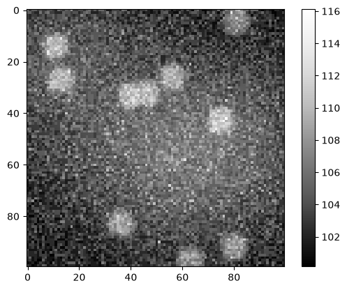
Image segmentation

If we now applied a segmentation algorithm to this image as it is, it might lead to a wrong result.

binary = cle.threshold_otsu(sum_image)

binary

cle._ image shape (100, 100) dtype uint8 size 9.8 kB min 0.0 max 1.0

Background removal

To fix this problem, we need to remove the background intensity first.

background_removed = cle.top_hat_box(sum_image, radius_x=10, radius_y=10)

background_removed

cle._ image shape (100, 100) dtype float32 size 39.1 kB min 0.0 max 12.833778381347656

Noise removal

We can also remove the noise from the image.

noise_removed1 = cle.mean_sphere(sum_image, radius_x=3, radius_y=3)

noise_removed1

cle._ image shape (100, 100) dtype float32 size 39.1 kB min 101.35627746582031 max 111.3677749633789

And this can also be done on the background-subtracted image.

noise_removed = cle.mean_sphere(background_removed, radius_x=3, radius_y=3)

noise_removed

cle._ image shape (100, 100) dtype float32 size 39.1 kB min 0.7578272223472595 max 7.551633834838867

Image segmentation II

After correcting the image, we can try segmentation again.

binary2 = cle.threshold_otsu(noise_removed)

binary2

cle._ image shape (100, 100) dtype uint8 size 9.8 kB min 0.0 max 1.0

# sneak preview: Voronoi-Labelling
labels = cle.voronoi_otsu_labeling(noise_removed, spot_sigma=1, outline_sigma=0)
labels

cle._ image shape (100, 100) dtype uint32 size 39.1 kB min 0.0 max 9.0

Exercise

Is the Difference of Gaussian a low-pass, high-pass or band-pass filter?

cle.difference_of_gaussian(sum_image,
                          sigma1_x=2,
                          sigma1_y=2,
                          sigma2_x=8,
                          sigma2_y=8,)

cle._ image shape (100, 100) dtype float32 size 39.1 kB min -1.332916259765625 max 3.963134765625