Visualization of measurements

In this notebook, we will analyze nuclei in a zebrafish eye image. The steps we plan to perform are:

1. Load the image data/zebrafish_eye.tif

2. Apply top-hat filtering with a radius of 15 to enhance nuclei (background subtraction)

3. Segment the nuclei using Voronoi-Otsu-labeling

4. Visualize the segmentation using an animated curtain overlay

5. Measure Feret’s diameter of each nucleus

6. Replace label values in the label image with their respective Feret’s diameter for visualization

Import Libraries

We import all necessary libraries for image loading, processing, segmentation, measurement, and visualization.

import numpy as np
import pandas as pd
import pyclesperanto as cle
import stackview
from skimage.io import imread
from skimage.measure import regionprops_table
import matplotlib.pyplot as plt

Step 1: Load the Image

We load the zebrafish eye image from disk and display it to get an overview of the data.

image = imread("data/zebrafish_eye.tif")

print("Image shape:", image.shape)
print("Image dtype:", image.dtype)
stackview.insight(image)

Image shape: (1024, 1024)
Image dtype: uint16

shape (1024, 1024) dtype uint16 size 2.0 MB min 3139 max 57638

Step 2: Apply Top-Hat Filtering

Top-hat filtering subtracts the background from the image, enhancing small bright structures such as nuclei. We use a radius of 15 pixels for the structuring element.

tophat_image = cle.top_hat(image, radius_x=15, radius_y=15, radius_z=15)

stackview.insight(tophat_image)

shape (1024, 1024) dtype float32 size 4.0 MB min 0.0 max 41810.0

Step 3: Segment Nuclei CellPose

We apply Voronoi-Otsu-labeling to the top-hat filtered image to detect and label individual nuclei. This method combines Gaussian spot detection with Otsu thresholding and Voronoi expansion.

from cellpose import models
model = models.CellposeModel(gpu=False)

100%|██████████| 1.15G/1.15G [00:40<00:00, 30.7MB/s]

label_image, _, _ = model.eval(image, 
                                  batch_size=32, 
                                  flow_threshold=0.4, 
                                  cellprob_threshold=0.0,
                                  normalize={"tile_norm_blocksize": 0})

# convert for better visualization
label_image = label_image.astype(np.uint32)

print("Number of detected nuclei:", int(label_image.max()))
stackview.insight(label_image)

Number of detected nuclei: 263

shape (1024, 1024) dtype uint32 size 4.0 MB min 0 max 263 n labels 263

Step 4: Visualize Segmentation with Animated Curtain

We use stackview.animate_curtain to display the original image alongside the segmentation label image in an animated blended overlay, allowing us to assess the quality of the segmentation.

stackview.animate_curtain(image, label_image)

C:\Users\haase\miniforge3\envs\bob-env\Lib\site-packages\stackview\_animate.py:63: UserWarning: The image is quite large (> 10 MByte) and might not be properly shown in the notebook when rendered over the internet. Consider subsampling or cropping the image for visualization purposes.
  warnings.warn("The image is quite large (> 10 MByte) and might not be properly shown in the notebook when rendered over the internet. Consider subsampling or cropping the image for visualization purposes.")

Step 5: Measure Feret’s Diameter of Nuclei

Feret’s diameter (the maximum caliper diameter) is a measure of the size of an object. We use skimage.measure.regionprops_table to measure the Feret’s diameter for each detected nucleus.

label_image_np = np.asarray(label_image)

properties = ['label', 'feret_diameter_max']
measurements = regionprops_table(label_image_np, properties=properties)
df = pd.DataFrame(measurements)

display(df.head())

	label	feret_diameter_max
0	1	46.043458
1	2	67.007462
2	3	56.824291
3	4	52.478567
4	5	58.180753

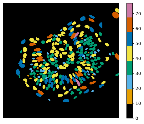
Step 6: Replace Labels with Feret’s Diameter for Visualization

To visualize the Feret’s diameter spatially, we replace each label in the label image with the corresponding Feret’s diameter value. This creates a parametric image where pixel intensity encodes the size of the nucleus. We use cle.replace_intensities for this purpose.

feret_map = cle.replace_intensities(label_image, [0] + df['feret_diameter_max'].tolist()).astype(np.float32)

stackview.imshow(feret_map, colormap="okabe_ito", colorbar=True)

Exercise

Visualize the area of the segmented cells.