This notebook may contain text, code and images generated by artificial intelligence. Used model: claude-sonnet-4-6, vision model: claude-sonnet-4-6, endpoint: None, bia-bob version: 0.34.3.. It is good scientific practice to check the code and results it produces carefully. Read more about code generation using bia-bob

Cell Rounding Assay Analysis

This notebook analyzes a timelapse microscopy dataset to track changes in cell shape over time using the aspect ratio (minor axis / major axis) as a measure of roundness. The dataset is a courtesy of Anne Esslinger, Alberti lab, MPI CBG.

import numpy as np
import pandas as pd
import matplotlib.pyplot as plt
import stackview
from skimage.io import imread
from skimage.measure import regionprops_table
from cellpose import models
from tqdm import tqdm

Load the Timelapse

We load the timelapse TIFF file and inspect its shape to understand the number of frames and image dimensions.

timelapse = imread("data/rounding_assay.tif")

# we only process a subsampled version of the image to avoid tiling artifacts
timelapse = timelapse[::2,::2,::2]

print("Shape:", timelapse.shape)
stackview.animate(timelapse)

Shape: (32, 256, 256)

Segmentation

For segmentation, we will use CellPose. We first initialize the model and then apply it to all frames individualy using a for-loop.

model = models.CellposeModel(gpu=False)
# see: torch.sparse.check_sparse_tensor_invariants.__doc__
import torch
torch.sparse.check_sparse_tensor_invariants.enable()

label_images = []

for i, frame in enumerate(tqdm(timelapse)):
    masks, flows, styles = model.eval(
        frame, 
        batch_size=32,
        flow_threshold=0.4,
        cellprob_threshold=0.0,
        normalize={"tile_norm_blocksize": 0}
    )
    label_images.append(masks.astype(np.uint32))

100%|██████████| 32/32 [01:26<00:00,  2.71s/it]

After segmentation, we can visualize the segmented label images over time.

stackview.animate(label_images)

Measurement

Next, we go through all segmented images using a for-loop to determine the aspect ratio. As scikit-image has no function for this, we need to compute the aspect-ratio ourselves from minor and major axis length of the objects.

avg_aspect_ratios = []

for i, label_image in enumerate(label_images):
    # measure
    props = regionprops_table(label_image, properties=['label', 'minor_axis_length', 'major_axis_length'])

    # convert to a Pandas DataFrame
    df = pd.DataFrame(props)

    # compute aspect ratio for each object
    df['aspect_ratio'] = df['minor_axis_length'] / df['major_axis_length']

    # compute the mean average aspect ratio for this frame
    avg_ar = df['aspect_ratio'].mean()

    # store result in a list
    avg_aspect_ratios.append(avg_ar)
    print(f"Frame {i}: avg aspect ratio = {avg_ar:.3f}")

Frame 0: avg aspect ratio = 0.352
Frame 1: avg aspect ratio = 0.377
Frame 2: avg aspect ratio = 0.377
Frame 3: avg aspect ratio = 0.404
Frame 4: avg aspect ratio = 0.417
Frame 5: avg aspect ratio = 0.440
Frame 6: avg aspect ratio = 0.515
Frame 7: avg aspect ratio = 0.542
Frame 8: avg aspect ratio = 0.544
Frame 9: avg aspect ratio = 0.569
Frame 10: avg aspect ratio = 0.574
Frame 11: avg aspect ratio = 0.605
Frame 12: avg aspect ratio = 0.618
Frame 13: avg aspect ratio = 0.615
Frame 14: avg aspect ratio = 0.656
Frame 15: avg aspect ratio = 0.752
Frame 16: avg aspect ratio = 0.780
Frame 17: avg aspect ratio = 0.772
Frame 18: avg aspect ratio = 0.757
Frame 19: avg aspect ratio = 0.793
Frame 20: avg aspect ratio = 0.810
Frame 21: avg aspect ratio = 0.832
Frame 22: avg aspect ratio = 0.840
Frame 23: avg aspect ratio = 0.847
Frame 24: avg aspect ratio = 0.841
Frame 25: avg aspect ratio = 0.845
Frame 26: avg aspect ratio = 0.851
Frame 27: avg aspect ratio = 0.858
Frame 28: avg aspect ratio = 0.824
Frame 29: avg aspect ratio = 0.858
Frame 30: avg aspect ratio = 0.860
Frame 31: avg aspect ratio = 0.869

Plotting

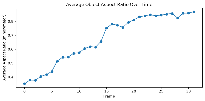
We plot the average aspect ratio across all frames to visualize how cell shape changes over the course of the experiment. A rising trend towards 1.0 indicates cells are becoming rounder.

plt.figure(figsize=(8, 4))
plt.plot(range(len(avg_aspect_ratios)), avg_aspect_ratios, marker='o')
plt.xlabel("Frame")
plt.ylabel("Average Aspect Ratio (minor/major)")
plt.title("Average Object Aspect Ratio Over Time")
plt.tight_layout()
plt.show()

Exercise

Duplicate this notebook. Then scroll up and comment out this line:

# timelapse = timelapse[::2,::2,::2]

Execute the entire notebook. What is different and why?