RandomForest with scikit-learn

RandomForest with scikit-learn#

We want to explore how to use scikit-learn for RandomForest. This includes preparing the data, training the model, and evaluating and visualizing the results.

We will use the following modules for this:

sklearn.datasets: Tools for using common datasets for ML or for generating synthetic data
sklearn.model_selection: Tools for data splitting, cross-validation, and parameter tuning
sklearn.tree and sklearn.ensemble: Collection of tree- and ensemble-based models for regression and classification
sklearn.metrics: Collection of various metrics for model evaluation

In general, also refer to the comprehensive User Guide on decision trees and User Guide on ensemble models from scikit-learn.

# Just in case we need help
# Import bia-bob as a helpful Python & Medical AI expert
from bia_bob import bob
import os

bob.initialize(
    endpoint='https://kiara.sc.uni-leipzig.de/api/v1', 
    model="vllm-llama-4-scout-17b-16e-instruct",
    system_prompt=os.getenv('SYSTEM_PROMPT_MEDICAL_AI')
)

This notebook may contain text, code and images generated by artificial intelligence. Used model: vllm-llama-4-scout-17b-16e-instruct, vision model: None, endpoint: https://kiara.sc.uni-leipzig.de/api/v1, bia-bob version: 0.34.3.. Do not enter sensitive or private information and verify generated contents according to good scientific practice. Read more: https://github.com/haesleinhuepf/bia-bob#disclaimer

%bob Who are you ? Just 1 sentence!

I’m a medical data science AI assistant, an expert in Python programming and data analysis, specializing in tasks like data preprocessing, feature engineering, machine learning, and deep learning for medical datasets.

RandomForest for Regression#

Data preparation#

Now we want to use a RandomForest to solve the regression problem for the scikit-learn diabetes dataset.

Let’s load the data again:

from sklearn.datasets import load_diabetes
diabetes = load_diabetes()

# Let's get our X,y first
X = diabetes.data
y = diabetes.target
# And here we also have proper labels for our features
feature_labels = diabetes.feature_names

print("Type X:", type(X))
print("Shape X:", X.shape)
print("First X:", X[0])
print("Labels X:", feature_labels)

Type X: <class 'numpy.ndarray'>
Shape X: (442, 10)
First X: [ 0.03807591  0.05068012  0.06169621  0.02187239 -0.0442235  -0.03482076
 -0.04340085 -0.00259226  0.01990749 -0.01764613]
Labels X: ['age', 'sex', 'bmi', 'bp', 's1', 's2', 's3', 's4', 's5', 's6']

print("Type y:", type(y))
print("Shape y:", y.shape)
print("First y:", y[0])

Type y: <class 'numpy.ndarray'>
Shape y: (442,)
First y: 151.0

Train-test split#

Now we split the data for training and model testing / evaluation in order to verify the generalization of the trained model on unknown data. For this purpose, we can use train_test_split.

from sklearn.model_selection import train_test_split

# Split: 80% training, 20% test
X_train, X_test, y_train, y_test = train_test_split(X, y, test_size=0.2, random_state=42)

print("training data:", X_train.shape, "training labels:", y_train.shape)
print("test data:", X_test.shape, "test labels:", y_test.shape)

training data: (353, 10) training labels: (353,)
test data: (89, 10) test labels: (89,)

Select and train a model#

We import the model RandomForestRegressor and initialize the corresponding Python object using () while also setting specific model parameters
Model training is started using the method .fit()
We pass the training data to this method, divided into features X_train and target y_train
The model parameters are now adjusted to predict the target as accurately as possible based on the associated feature

from sklearn.ensemble import RandomForestRegressor

# Initialize model with model parameters
# - n_estimators: number of decision trees in the forest
# - max_depth: maximum depth of a tree
model = RandomForestRegressor(
    n_estimators=5,
    max_depth=None
)

# Supervised training - “Fitting” the model to the training data with known labels
model.fit(X_train, y_train)

RandomForestRegressor(n_estimators=5)

In a Jupyter environment, please rerun this cell to show the HTML representation or trust the notebook.
On GitHub, the HTML representation is unable to render, please try loading this page with nbviewer.org.

Prediction and evaluation#

We now want to check how well the model can predict the target for previously unknown features.

The prediction is performed using the method .predict() – almost all models and algorithms in scikit-learn have this method.
We pass the features of the test data to this method and receive the corresponding predictions of the target.

# Prediction on unseen test data
y_pred = model.predict(X_test)

We can now compare the predictions with the known target values of the test data and derive metrics for evaluating the model quality.

A metric provided by RandomForestRegressor itself is the so-called r2 score (coefficient of determination of a regression), which evaluates the overall goodness of fit
Other suitable regression metrics are described, for example, in the User Guide - Regression Metrics
We also choose the Mean Absolute Error (MAE)
In general, it makes sense to calculate several metrics in order to get a better impression of the model quality

from sklearn.metrics import mean_absolute_error

# Metrics for determining model quality

# r^2 score, between 0.0 and 1.0, higher is better
r2_score = model.score(X_test, y_test)
print(f"r^2 score on test data: {r2_score:.3f}")

# Calculate mean absolute error (MAE), the best is 0.0
mse = mean_absolute_error(y_test, y_pred)
print(f"Mean Absolute Error (MAE) on test data: {mse:.3f}")

r^2 score on test data: 0.379
Mean Absolute Error (MAE) on test data: 47.007

Parameter tuning#

At the moment, we have simply estimated the values for the model parameters n_estimators and max_depth and obtained an evaluation result for this combination. But how can we be sure that this is actually the best choice, or whether we can still improve the model quality?

# We can check all available parameters again
model.get_params()

{'bootstrap': True,
 'ccp_alpha': 0.0,
 'criterion': 'squared_error',
 'max_depth': None,
 'max_features': 1.0,
 'max_leaf_nodes': None,
 'max_samples': None,
 'min_impurity_decrease': 0.0,
 'min_samples_leaf': 1,
 'min_samples_split': 2,
 'min_weight_fraction_leaf': 0.0,
 'monotonic_cst': None,
 'n_estimators': 5,
 'n_jobs': None,
 'oob_score': False,
 'random_state': None,
 'verbose': 0,
 'warm_start': False}

Since trial and error would be very time-consuming with a large number of available parameters and combinations, we should use an automated approach that employs scikit-learn hyper-parameter tuning methods.

We want to apply a basic grid search over specified parameter values using sklearn.model_selection.GridSearchCV

from sklearn.model_selection import GridSearchCV

# Define the parameter grid we want to search
param_grid = {
    'n_estimators': [1, 25, 50, 200],
    'max_depth': [None, 5, 25, 50],
}

# Initialize GridSearchCV with the following parameters
# - estimator: the model we want to tune
# - param_grid: the parameter grid to search from
# - scoring: score used to determine the model quality for given parameters
# - cv: cross-validation data splitting strategy (n-fold)
grid_search = GridSearchCV(
    estimator=RandomForestRegressor(random_state=42),
    param_grid=param_grid,
    scoring='r2',
    cv=5
)

# Perform grid search, may take a while
grid_search.fit(X_train, y_train)

GridSearchCV(cv=5, estimator=RandomForestRegressor(random_state=42),
             param_grid={'max_depth': [None, 5, 25, 50],
                         'n_estimators': [1, 25, 50, 200]},
             scoring='r2')

In a Jupyter environment, please rerun this cell to show the HTML representation or trust the notebook.
On GitHub, the HTML representation is unable to render, please try loading this page with nbviewer.org.

# Print best parameter combination with the best score
print("Best parameters for training data:", grid_search.best_params_)
print("Best score for training data:", grid_search.best_score_)

# Get the best model with the best parameter choice
best_model = grid_search.best_estimator_

Best parameters for training data: {'max_depth': 5, 'n_estimators': 200}
Best score for training data: 0.40719110568079026

As we can see, setting max_depth=5 and n_estimators=200 delivered the best results for the training data.

Let’s evaluate the predictions of this best model with our test data.

# Prediction on unseen test data
y_pred_best = best_model.predict(X_test)

# r^2 score, between 0.0 and 1.0, higher is better
r2_score = best_model.score(X_test, y_test)
print(f"r^2 score on test data: {r2_score:.3f}")

# Calculate mean absolute error (MAE), the best is 0.0
mse = mean_absolute_error(y_test, y_pred_best)
print(f"Mean Absolute Error (MAE) on test data: {mse:.3f}")

r^2 score on test data: 0.460
Mean Absolute Error (MAE) on test data: 43.274

Explainability#

Tree insights#

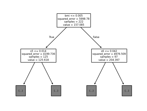
Now that we have trees built inside our RandomForest, we can examine separate trees by plotting them.

from sklearn import tree

# Plot the first tree from our RandomForest with limited depth
tree.plot_tree(best_model.estimators_[0],
               max_depth=1,
               feature_names = feature_labels)

[Text(0.5, 0.8333333333333334, 'bmi <= 0.005\nsquared_error = 5998.78\nsamples = 222\nvalue = 157.085'),
 Text(0.25, 0.5, 's5 <= 0.014\nsquared_error = 4199.736\nsamples = 125\nvalue = 125.618'),
 Text(0.375, 0.6666666666666667, 'True  '),
 Text(0.125, 0.16666666666666666, '\n  (...)  \n'),
 Text(0.375, 0.16666666666666666, '\n  (...)  \n'),
 Text(0.75, 0.5, 's6 <= 0.042\nsquared_error = 4976.509\nsamples = 97\nvalue = 204.397'),
 Text(0.625, 0.6666666666666667, '  False'),
 Text(0.625, 0.16666666666666666, '\n  (...)  \n'),
 Text(0.875, 0.16666666666666666, '\n  (...)  \n')]

../_images/a00fae8413259d79986f75d525f0000fb8254202438503b067a3cd51212d1388.png

Feature importance#

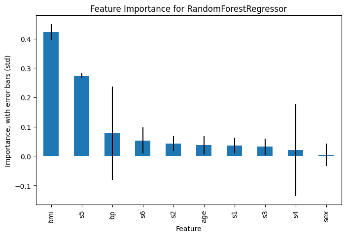
Now that we have an example with more than one feature, we can also evaluate the significance / importance of the features for the regression task. This helps to understand which features contributed to the prediction and to what extent. This information can then be used for a more refind feature selection.

For this, some models in scikit-learn provide the attribute feature_importances_ (impurity-based, good for low cardinality features). In addition, the more sophisticated method sklearn.inspection.permutation_importance is available.

import numpy as np
import pandas as pd

# Extract feature importances from the best model, store sorted in a pandas Series
importances = pd.Series(best_model.feature_importances_, index=feature_labels).sort_values(ascending=False)

# Get the standard deviations of importances across trees as a measure of the variability
importances_std = np.std([tree.feature_importances_ for tree in best_model.estimators_], axis=0)

Now we can plot the feature importances, including the standard deviations as error bars

import matplotlib.pyplot as plt

plt.figure(figsize=(8, 5))
importances.plot(kind='bar', yerr=importances_std)
plt.xlabel('Feature')
plt.ylabel('Importance, with error bars (std)')
plt.title('Feature Importance for RandomForestRegressor')
plt.show()

../_images/7f9c75fea36b9176296b924e28b1d4cb34a038b21d70c5a48d53a63d64075b75.png

Exercise: Classification with RandomForest#

Now it’s your turn to apply a RandomForest to a classification problem, using the scikit-learn breast cancer diagnostic dataset.

This data contains features computed from 569 digitized images of a breast mass, which shall be used to predict two classes: WDBC-Malignant, or WDBC-Benign.

For example, you can use the following objects and methods:

RandomForestClassifier as model
GridSearchCV or RandomizedSearchCV for parameter optimization
Classification Metrics to evaluate the model quality
permutation_importance for explainability

If you get stuck, remember that our assistant bia-bob is available and very happy to help you.

Data preparation#

from sklearn.datasets import load_breast_cancer

breast_cancer = load_breast_cancer()
dir(breast_cancer)

['DESCR',
 'data',
 'data_module',
 'feature_names',
 'filename',
 'frame',
 'target',
 'target_names']

# ToDo: understand the data better

Train-test split#

# ToDo: create data for training and test

Select and train a model#

# ToDo: initialize and train a classification model with parameter optimization

Prediction and evaluation#

# ToDo: evaluate the model quality

	n_estimators n_estimators: int, default=100 The number of trees in the forest. .. versionchanged:: 0.22 The default value of ``n_estimators`` changed from 10 to 100 in 0.22.	5
	criterion criterion: {"squared_error", "absolute_error", "friedman_mse", "poisson"}, default="squared_error" The function to measure the quality of a split. Supported criteria are "squared_error" for the mean squared error, which is equal to variance reduction as feature selection criterion and minimizes the L2 loss using the mean of each terminal node, "friedman_mse", which uses mean squared error with Friedman's improvement score for potential splits, "absolute_error" for the mean absolute error, which minimizes the L1 loss using the median of each terminal node, and "poisson" which uses reduction in Poisson deviance to find splits. Training using "absolute_error" is significantly slower than when using "squared_error". .. versionadded:: 0.18 Mean Absolute Error (MAE) criterion. .. versionadded:: 1.0 Poisson criterion.	'squared_error'
	max_depth max_depth: int, default=None The maximum depth of the tree. If None, then nodes are expanded until all leaves are pure or until all leaves contain less than min_samples_split samples.	None
	min_samples_split min_samples_split: int or float, default=2 The minimum number of samples required to split an internal node: - If int, then consider `min_samples_split` as the minimum number. - If float, then `min_samples_split` is a fraction and `ceil(min_samples_split * n_samples)` are the minimum number of samples for each split. .. versionchanged:: 0.18 Added float values for fractions.	2
	min_samples_leaf min_samples_leaf: int or float, default=1 The minimum number of samples required to be at a leaf node. A split point at any depth will only be considered if it leaves at least ``min_samples_leaf`` training samples in each of the left and right branches. This may have the effect of smoothing the model, especially in regression. - If int, then consider `min_samples_leaf` as the minimum number. - If float, then `min_samples_leaf` is a fraction and `ceil(min_samples_leaf * n_samples)` are the minimum number of samples for each node. .. versionchanged:: 0.18 Added float values for fractions.	1
	min_weight_fraction_leaf min_weight_fraction_leaf: float, default=0.0 The minimum weighted fraction of the sum total of weights (of all the input samples) required to be at a leaf node. Samples have equal weight when sample_weight is not provided.	0.0
	max_features max_features: {"sqrt", "log2", None}, int or float, default=1.0 The number of features to consider when looking for the best split: - If int, then consider `max_features` features at each split. - If float, then `max_features` is a fraction and `max(1, int(max_features * n_features_in_))` features are considered at each split. - If "sqrt", then `max_features=sqrt(n_features)`. - If "log2", then `max_features=log2(n_features)`. - If None or 1.0, then `max_features=n_features`. .. note:: The default of 1.0 is equivalent to bagged trees and more randomness can be achieved by setting smaller values, e.g. 0.3. .. versionchanged:: 1.1 The default of `max_features` changed from `"auto"` to 1.0. Note: the search for a split does not stop until at least one valid partition of the node samples is found, even if it requires to effectively inspect more than ``max_features`` features.	1.0
	max_leaf_nodes max_leaf_nodes: int, default=None Grow trees with ``max_leaf_nodes`` in best-first fashion. Best nodes are defined as relative reduction in impurity. If None then unlimited number of leaf nodes.	None
	min_impurity_decrease min_impurity_decrease: float, default=0.0 A node will be split if this split induces a decrease of the impurity greater than or equal to this value. The weighted impurity decrease equation is the following:: N_t / N * (impurity - N_t_R / N_t * right_impurity - N_t_L / N_t * left_impurity) where ``N`` is the total number of samples, ``N_t`` is the number of samples at the current node, ``N_t_L`` is the number of samples in the left child, and ``N_t_R`` is the number of samples in the right child. ``N``, ``N_t``, ``N_t_R`` and ``N_t_L`` all refer to the weighted sum, if ``sample_weight`` is passed. .. versionadded:: 0.19	0.0
	bootstrap bootstrap: bool, default=True Whether bootstrap samples are used when building trees. If False, the whole dataset is used to build each tree.	True
	oob_score oob_score: bool or callable, default=False Whether to use out-of-bag samples to estimate the generalization score. By default, :func:`~sklearn.metrics.r2_score` is used. Provide a callable with signature `metric(y_true, y_pred)` to use a custom metric. Only available if `bootstrap=True`. For an illustration of out-of-bag (OOB) error estimation, see the example :ref:`sphx_glr_auto_examples_ensemble_plot_ensemble_oob.py`.	False
	n_jobs n_jobs: int, default=None The number of jobs to run in parallel. :meth:`fit`, :meth:`predict`, :meth:`decision_path` and :meth:`apply` are all parallelized over the trees. ``None`` means 1 unless in a :obj:`joblib.parallel_backend` context. ``-1`` means using all processors. See :term:`Glossary ` for more details.	None
	random_state random_state: int, RandomState instance or None, default=None Controls both the randomness of the bootstrapping of the samples used when building trees (if ``bootstrap=True``) and the sampling of the features to consider when looking for the best split at each node (if ``max_features < n_features``). See :term:`Glossary ` for details.	None
	verbose verbose: int, default=0 Controls the verbosity when fitting and predicting.	0
	warm_start warm_start: bool, default=False When set to ``True``, reuse the solution of the previous call to fit and add more estimators to the ensemble, otherwise, just fit a whole new forest. See :term:`Glossary ` and :ref:`tree_ensemble_warm_start` for details.	False
	ccp_alpha ccp_alpha: non-negative float, default=0.0 Complexity parameter used for Minimal Cost-Complexity Pruning. The subtree with the largest cost complexity that is smaller than ``ccp_alpha`` will be chosen. By default, no pruning is performed. See :ref:`minimal_cost_complexity_pruning` for details. See :ref:`sphx_glr_auto_examples_tree_plot_cost_complexity_pruning.py` for an example of such pruning. .. versionadded:: 0.22	0.0
	max_samples max_samples: int or float, default=None If bootstrap is True, the number of samples to draw from X to train each base estimator. - If None (default), then draw `X.shape[0]` samples. - If int, then draw `max_samples` samples. - If float, then draw `max(round(n_samples * max_samples), 1)` samples. Thus, `max_samples` should be in the interval `(0.0, 1.0]`. .. versionadded:: 0.22	None
	monotonic_cst monotonic_cst: array-like of int of shape (n_features), default=None Indicates the monotonicity constraint to enforce on each feature. - 1: monotonically increasing - 0: no constraint - -1: monotonically decreasing If monotonic_cst is None, no constraints are applied. Monotonicity constraints are not supported for: - multioutput regressions (i.e. when `n_outputs_ > 1`), - regressions trained on data with missing values. Read more in the :ref:`User Guide `. .. versionadded:: 1.4	None

	estimator estimator: estimator object This is assumed to implement the scikit-learn estimator interface. Either estimator needs to provide a ``score`` function, or ``scoring`` must be passed.	RandomForestR...ndom_state=42)
	param_grid param_grid: dict or list of dictionaries Dictionary with parameters names (`str`) as keys and lists of parameter settings to try as values, or a list of such dictionaries, in which case the grids spanned by each dictionary in the list are explored. This enables searching over any sequence of parameter settings.	{'max_depth': [None, 5, ...], 'n_estimators': [1, 25, ...]}
	scoring scoring: str, callable, list, tuple or dict, default=None Strategy to evaluate the performance of the cross-validated model on the test set. If `scoring` represents a single score, one can use: - a single string (see :ref:`scoring_string_names`); - a callable (see :ref:`scoring_callable`) that returns a single value; - `None`, the `estimator`'s :ref:`default evaluation criterion ` is used. If `scoring` represents multiple scores, one can use: - a list or tuple of unique strings; - a callable returning a dictionary where the keys are the metric names and the values are the metric scores; - a dictionary with metric names as keys and callables as values. See :ref:`multimetric_grid_search` for an example.	'r2'
	n_jobs n_jobs: int, default=None Number of jobs to run in parallel. ``None`` means 1 unless in a :obj:`joblib.parallel_backend` context. ``-1`` means using all processors. See :term:`Glossary ` for more details. .. versionchanged:: v0.20 `n_jobs` default changed from 1 to None	None
	refit refit: bool, str, or callable, default=True Refit an estimator using the best found parameters on the whole dataset. For multiple metric evaluation, this needs to be a `str` denoting the scorer that would be used to find the best parameters for refitting the estimator at the end. Where there are considerations other than maximum score in choosing a best estimator, ``refit`` can be set to a function which returns the selected ``best_index_`` given ``cv_results_``. In that case, the ``best_estimator_`` and ``best_params_`` will be set according to the returned ``best_index_`` while the ``best_score_`` attribute will not be available. The refitted estimator is made available at the ``best_estimator_`` attribute and permits using ``predict`` directly on this ``GridSearchCV`` instance. Also for multiple metric evaluation, the attributes ``best_index_``, ``best_score_`` and ``best_params_`` will only be available if ``refit`` is set and all of them will be determined w.r.t this specific scorer. See ``scoring`` parameter to know more about multiple metric evaluation. See :ref:`sphx_glr_auto_examples_model_selection_plot_grid_search_digits.py` to see how to design a custom selection strategy using a callable via `refit`. See :ref:`this example ` for an example of how to use ``refit=callable`` to balance model complexity and cross-validated score. .. versionchanged:: 0.20 Support for callable added.	True
	cv cv: int, cross-validation generator or an iterable, default=None Determines the cross-validation splitting strategy. Possible inputs for cv are: - None, to use the default 5-fold cross validation, - integer, to specify the number of folds in a `(Stratified)KFold`, - :term:`CV splitter`, - An iterable yielding (train, test) splits as arrays of indices. For integer/None inputs, if the estimator is a classifier and ``y`` is either binary or multiclass, :class:`StratifiedKFold` is used. In all other cases, :class:`KFold` is used. These splitters are instantiated with `shuffle=False` so the splits will be the same across calls. Refer :ref:`User Guide ` for the various cross-validation strategies that can be used here. .. versionchanged:: 0.22 ``cv`` default value if None changed from 3-fold to 5-fold.	5
	verbose verbose: int Controls the verbosity: the higher, the more messages. - >1 : the computation time for each fold and parameter candidate is displayed; - >2 : the score is also displayed; - >3 : the fold and candidate parameter indexes are also displayed together with the starting time of the computation.	0
	pre_dispatch pre_dispatch: int, or str, default='2n_jobs' Controls the number of jobs that get dispatched during parallel execution. Reducing this number can be useful to avoid an explosion of memory consumption when more jobs get dispatched than CPUs can process. This parameter can be: - None, in which case all the jobs are immediately created and spawned. Use this for lightweight and fast-running jobs, to avoid delays due to on-demand spawning of the jobs - An int, giving the exact number of total jobs that are spawned - A str, giving an expression as a function of n_jobs, as in '2n_jobs'	'2*n_jobs'
	error_score error_score: 'raise' or numeric, default=np.nan Value to assign to the score if an error occurs in estimator fitting. If set to 'raise', the error is raised. If a numeric value is given, FitFailedWarning is raised. This parameter does not affect the refit step, which will always raise the error.	nan
	return_train_score return_train_score: bool, default=False If ``False``, the ``cv_results_`` attribute will not include training scores. Computing training scores is used to get insights on how different parameter settings impact the overfitting/underfitting trade-off. However computing the scores on the training set can be computationally expensive and is not strictly required to select the parameters that yield the best generalization performance. .. versionadded:: 0.19 .. versionchanged:: 0.21 Default value was changed from ``True`` to ``False``	False

	n_estimators n_estimators: int, default=100 The number of trees in the forest. .. versionchanged:: 0.22 The default value of ``n_estimators`` changed from 10 to 100 in 0.22.	200
	criterion criterion: {"squared_error", "absolute_error", "friedman_mse", "poisson"}, default="squared_error" The function to measure the quality of a split. Supported criteria are "squared_error" for the mean squared error, which is equal to variance reduction as feature selection criterion and minimizes the L2 loss using the mean of each terminal node, "friedman_mse", which uses mean squared error with Friedman's improvement score for potential splits, "absolute_error" for the mean absolute error, which minimizes the L1 loss using the median of each terminal node, and "poisson" which uses reduction in Poisson deviance to find splits. Training using "absolute_error" is significantly slower than when using "squared_error". .. versionadded:: 0.18 Mean Absolute Error (MAE) criterion. .. versionadded:: 1.0 Poisson criterion.	'squared_error'
	max_depth max_depth: int, default=None The maximum depth of the tree. If None, then nodes are expanded until all leaves are pure or until all leaves contain less than min_samples_split samples.	5
	min_samples_split min_samples_split: int or float, default=2 The minimum number of samples required to split an internal node: - If int, then consider `min_samples_split` as the minimum number. - If float, then `min_samples_split` is a fraction and `ceil(min_samples_split * n_samples)` are the minimum number of samples for each split. .. versionchanged:: 0.18 Added float values for fractions.	2
	min_samples_leaf min_samples_leaf: int or float, default=1 The minimum number of samples required to be at a leaf node. A split point at any depth will only be considered if it leaves at least ``min_samples_leaf`` training samples in each of the left and right branches. This may have the effect of smoothing the model, especially in regression. - If int, then consider `min_samples_leaf` as the minimum number. - If float, then `min_samples_leaf` is a fraction and `ceil(min_samples_leaf * n_samples)` are the minimum number of samples for each node. .. versionchanged:: 0.18 Added float values for fractions.	1
	min_weight_fraction_leaf min_weight_fraction_leaf: float, default=0.0 The minimum weighted fraction of the sum total of weights (of all the input samples) required to be at a leaf node. Samples have equal weight when sample_weight is not provided.	0.0
	max_features max_features: {"sqrt", "log2", None}, int or float, default=1.0 The number of features to consider when looking for the best split: - If int, then consider `max_features` features at each split. - If float, then `max_features` is a fraction and `max(1, int(max_features * n_features_in_))` features are considered at each split. - If "sqrt", then `max_features=sqrt(n_features)`. - If "log2", then `max_features=log2(n_features)`. - If None or 1.0, then `max_features=n_features`. .. note:: The default of 1.0 is equivalent to bagged trees and more randomness can be achieved by setting smaller values, e.g. 0.3. .. versionchanged:: 1.1 The default of `max_features` changed from `"auto"` to 1.0. Note: the search for a split does not stop until at least one valid partition of the node samples is found, even if it requires to effectively inspect more than ``max_features`` features.	1.0
	max_leaf_nodes max_leaf_nodes: int, default=None Grow trees with ``max_leaf_nodes`` in best-first fashion. Best nodes are defined as relative reduction in impurity. If None then unlimited number of leaf nodes.	None
	min_impurity_decrease min_impurity_decrease: float, default=0.0 A node will be split if this split induces a decrease of the impurity greater than or equal to this value. The weighted impurity decrease equation is the following:: N_t / N * (impurity - N_t_R / N_t * right_impurity - N_t_L / N_t * left_impurity) where ``N`` is the total number of samples, ``N_t`` is the number of samples at the current node, ``N_t_L`` is the number of samples in the left child, and ``N_t_R`` is the number of samples in the right child. ``N``, ``N_t``, ``N_t_R`` and ``N_t_L`` all refer to the weighted sum, if ``sample_weight`` is passed. .. versionadded:: 0.19	0.0
	bootstrap bootstrap: bool, default=True Whether bootstrap samples are used when building trees. If False, the whole dataset is used to build each tree.	True
	oob_score oob_score: bool or callable, default=False Whether to use out-of-bag samples to estimate the generalization score. By default, :func:`~sklearn.metrics.r2_score` is used. Provide a callable with signature `metric(y_true, y_pred)` to use a custom metric. Only available if `bootstrap=True`. For an illustration of out-of-bag (OOB) error estimation, see the example :ref:`sphx_glr_auto_examples_ensemble_plot_ensemble_oob.py`.	False
	n_jobs n_jobs: int, default=None The number of jobs to run in parallel. :meth:`fit`, :meth:`predict`, :meth:`decision_path` and :meth:`apply` are all parallelized over the trees. ``None`` means 1 unless in a :obj:`joblib.parallel_backend` context. ``-1`` means using all processors. See :term:`Glossary ` for more details.	None
	random_state random_state: int, RandomState instance or None, default=None Controls both the randomness of the bootstrapping of the samples used when building trees (if ``bootstrap=True``) and the sampling of the features to consider when looking for the best split at each node (if ``max_features < n_features``). See :term:`Glossary ` for details.	42
	verbose verbose: int, default=0 Controls the verbosity when fitting and predicting.	0
	warm_start warm_start: bool, default=False When set to ``True``, reuse the solution of the previous call to fit and add more estimators to the ensemble, otherwise, just fit a whole new forest. See :term:`Glossary ` and :ref:`tree_ensemble_warm_start` for details.	False
	ccp_alpha ccp_alpha: non-negative float, default=0.0 Complexity parameter used for Minimal Cost-Complexity Pruning. The subtree with the largest cost complexity that is smaller than ``ccp_alpha`` will be chosen. By default, no pruning is performed. See :ref:`minimal_cost_complexity_pruning` for details. See :ref:`sphx_glr_auto_examples_tree_plot_cost_complexity_pruning.py` for an example of such pruning. .. versionadded:: 0.22	0.0
	max_samples max_samples: int or float, default=None If bootstrap is True, the number of samples to draw from X to train each base estimator. - If None (default), then draw `X.shape[0]` samples. - If int, then draw `max_samples` samples. - If float, then draw `max(round(n_samples * max_samples), 1)` samples. Thus, `max_samples` should be in the interval `(0.0, 1.0]`. .. versionadded:: 0.22	None
	monotonic_cst monotonic_cst: array-like of int of shape (n_features), default=None Indicates the monotonicity constraint to enforce on each feature. - 1: monotonically increasing - 0: no constraint - -1: monotonically decreasing If monotonic_cst is None, no constraints are applied. Monotonicity constraints are not supported for: - multioutput regressions (i.e. when `n_outputs_ > 1`), - regressions trained on data with missing values. Read more in the :ref:`User Guide `. .. versionadded:: 1.4	None

RandomForest with scikit-learn

Contents

RandomForest with scikit-learn#

RandomForest for Regression#

Data preparation#

Train-test split#

Select and train a model#

Prediction and evaluation#

Parameter tuning#

Explainability#

Tree insights#

Feature importance#

Exercise: Classification with RandomForest#

Data preparation#

Train-test split#

Select and train a model#

Prediction and evaluation#