Clustering with scikit-learn

Clustering with scikit-learn#

We want to explore how to use scikit-learn for clustering. This includes preparing the data, training the model, and evaluating and visualizing the results.

We will use the following modules for this:

sklearn.datasets: Tools for using common datasets for ML or for generating synthetic data
sklearn.model_selection: Tools for data splitting, cross-validation, and parameter tuning
sklearn.cluster: Collection of clustering models
sklearn.metrics: Collection of various metrics for model evaluation

In general, also refer to the comprehensive User Guide on clustering from scikit-learn.

# Just in case we need help
# Import bia-bob as a helpful Python & Medical AI expert
from bia_bob import bob
import os

bob.initialize(
    endpoint='https://kiara.sc.uni-leipzig.de/api/v1', 
    model="vllm-llama-4-scout-17b-16e-instruct",
    system_prompt=os.getenv('SYSTEM_PROMPT_MEDICAL_AI')
)

This notebook may contain text, code and images generated by artificial intelligence. Used model: vllm-llama-4-scout-17b-16e-instruct, vision model: None, endpoint: https://kiara.sc.uni-leipzig.de/api/v1, bia-bob version: 0.34.3.. Do not enter sensitive or private information and verify generated contents according to good scientific practice. Read more: https://github.com/haesleinhuepf/bia-bob#disclaimer

%bob Who are you ? Just 1 sentence!

I’m a medical data science AI assistant, an expert in Python programming and data analysis with extensive experience working with various medical datasets.

Clustering on synthetic data#

Data preparation#

For a start and to show the concepts of clustering with scikit-learn, we generate synthetic data for a simple clustering problem.
We use make_blobs:

To get 100 data points (samples) with 5 features each in X,
With data points divided in 4 classes in y
And an increased standard deviation in the classes for a more scattered distribution

from sklearn.datasets import make_blobs

# We use the established notation: X for Features, y for Target
X, y = make_blobs(
    n_samples=100,
    n_features=5,
    centers=4,
    cluster_std=3,
    random_state=42
)

print("Type X:", type(X))
print("Shape X:", X.shape)
print("First X:", X[0])
print("Type y:", type(y))
print("Shape y:", y.shape)
print("First y:", y[0])

Type X: <class 'numpy.ndarray'>
Shape X: (100, 5)
First X: [-0.60365988 -8.11085786  2.18403634 -3.31302733 -5.63679335]
Type y: <class 'numpy.ndarray'>
Shape y: (100,)
First y: 3

To make the data a little more convenient to work with, we load it into a pandas dataframe, and use pandas’ methods to get a better overview on the data.

import pandas as pd

df = pd.DataFrame(X, columns=[f'feature_{i}' for i in range(0, X.shape[1])])
df['target'] = y

df.info()

<class 'pandas.core.frame.DataFrame'>
RangeIndex: 100 entries, 0 to 99
Data columns (total 6 columns):
 #   Column     Non-Null Count  Dtype  
---  ------     --------------  -----  
 0   feature_0  100 non-null    float64
 1   feature_1  100 non-null    float64
 2   feature_2  100 non-null    float64
 3   feature_3  100 non-null    float64
 4   feature_4  100 non-null    float64
 5   target     100 non-null    int64  
dtypes: float64(5), int64(1)
memory usage: 4.8 KB

df.describe().T

	count	mean	std	min	25%	50%	75%	max
feature_0	100.0	-6.087772	3.744947	-13.932563	-8.934807	-5.901472	-3.471680	3.149360
feature_1	100.0	1.008372	8.795885	-18.562130	-7.194092	1.586486	9.102682	15.026710
feature_2	100.0	5.177931	3.659623	-4.615019	2.790411	5.333441	7.920806	13.218262
feature_3	100.0	-0.895574	4.427548	-8.771270	-3.898520	-0.618707	2.399723	13.580495
feature_4	100.0	-3.381674	5.288010	-12.635941	-6.850471	-4.821894	0.622928	11.105427
target	100.0	1.500000	1.123666	0.000000	0.750000	1.500000	2.250000	3.000000

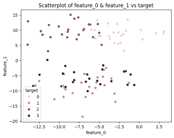
Visualizing 5-dimensional data (5 features) is not really possible.
So let’s visualize just 2 of the features (2 dimensions of the data) vs. the target in a 2D scatterplot.

import seaborn as sns
import matplotlib.pyplot as plt

sns.scatterplot(data=df, x=df.columns[0], y=df.columns[1], hue='target')
plt.title(f'Scatterplot of {df.columns[0]} & {df.columns[1]} vs target')
plt.show()

../_images/e8905955580c9b9d279a87a1beb55c4391975c9205a9c5bf32b1a7b19954a218.png

Data Scaling#

As we can see from the descriptive statistics above, the features have different means, standard deviations, and numeric ranges. Distance-based clustering algorithms, like KMeans, compute distances between data points. Features with larger numeric ranges can dominate the distance measure and disproportionately influence the clustering result, even if they are not inherently more important. Scaling ensures that all features contribute more equally.

Depending on the data, there are various methods for doing this, like described in the User Guide on data processing, or in the Examples on preprocessing.

We will use the StandardScaler, which works well for data without outliers, and scales the features to have zero mean and unit variance.

from sklearn.preprocessing import StandardScaler

scaler = StandardScaler().fit(X)
X_scaled = scaler.transform(X)

df_scaled = pd.DataFrame(X_scaled, columns=[f'feature_{i}' for i in range(0, X.shape[1])])
df_scaled['target'] = y

df_scaled.describe().T

	count	mean	std	min	25%	50%	75%	max
feature_0	100.0	-1.154632e-16	1.005038	-2.105320	-0.764064	0.049998	0.702085	2.478985
feature_1	100.0	1.887379e-17	1.005038	-2.236170	-0.937232	0.066057	0.924874	1.601767
feature_2	100.0	2.386980e-17	1.005038	-2.689426	-0.655682	0.042708	0.753273	2.208106
feature_3	100.0	2.886580e-17	1.005038	-1.787755	-0.681658	0.062848	0.748021	3.286016
feature_4	100.0	-2.070566e-16	1.005038	-1.758864	-0.659279	-0.273728	0.761114	2.753415
target	100.0	1.500000e+00	1.123666	0.000000	0.750000	1.500000	2.250000	3.000000

Select and train a model#

We want to make use of the basic KMeans clustering algorithm.
For clustering, we do not necessarely need to split our data for training and test.

We import the model KMeans and initialize the corresponding Python object using () while also setting specific model parameters
Model training is started using the method .fit_predict()
We pass the data as a whole to this method
The model parameters are now adjusted to predict the target (clusters) as accurately as possible based on the associated feature

from sklearn.cluster import KMeans

# Initialize model with model parameters
# - n_clusters: number of expected clusters 
#   -> since we do not know any better yet, we assume it may be 2
model = KMeans(
    n_clusters=2
)

# Unsupervised training 
# - “Fitting” the model to the training data without known labels
# - return the estimated cluster assignments for the samples
y_pred = model.fit_predict(X_scaled)

Evaluation#

We now want to check how well the model can predict the actual clusters for our data by comparing the predictions with the known classes derive metrics for evaluating the model quality.

Suitable clustering metrics are described, e.g., in the User Guide - Clustering Evaluation
We choose
- Silhouette Coefficient:
  - The score is bounded between -1 for incorrect clustering and +1 for highly dense clustering. Scores around zero indicate overlapping clusters.
  - The score is higher when clusters are dense and well separated, which relates to a standard concept of a cluster.
- Homogeneity-Completeness measures:
  - Homogeneity and Completeness are bounded below by 0.0 and above by 1.0 (higher is better)
  - V-measure is the harmonic mean of both
In general, it makes sense to calculate several metrics in order to get a better impression of the model quality

from sklearn.metrics import homogeneity_completeness_v_measure, silhouette_score

sc = silhouette_score(X_scaled, y_pred, metric='euclidean')
hcv = homogeneity_completeness_v_measure(y, y_pred)

print('silhouette_score: ', sc)
print('homogeneity_completeness_v_measure: ', hcv)

silhouette_score:  0.281290416197809
homogeneity_completeness_v_measure:  (0.3452593775422309, 0.7635259980029555, 0.4755014209638048)

Parameter tuning#

We did run the KMeans clustering under the assumption there may be 2 clusters. For KMeans, this value is a model parameter. And we can try other values to see whether the metrics for evaluation, i.e., the clustering quality may improve.

Exercise#

Now it’s your turn! Check for different values for the parameter n_clusters to see if the values of the evaluation metrics can be improved. The goal is to find the value for n_clusters that achieves the best evaluation result for both silhouette_score and v_measure. Plotting the evaluation metrics may help to get a better impression.

Hint: a loop is the easiest approach

You may ask our assistant bia-bob for help.

# ToDo: Parameter tuning for KMeans

Cluster Analysis#

Now that we have our original data and the cluster assignments predicted by the clustering algorithm, we can explore the clusters in more detail. For example, we can compute the mean value of each feature per cluster to get an idea of how the clusters differ.

Since the row order of X (our original data) and y_pred (the predicted cluster labels) is the same, we can combine them into a single DataFrame. Then we can use groupby to aggregate the feature values cluster-wise.

This gives us a simple way to interpret the clustering result by summarizing each cluster with descriptive statistics.

df_results = pd.DataFrame(X, columns=[f'feature_{i}' for i in range(0, X.shape[1])])
df_results['predicted_cluster'] = y_pred

# ToDo