Neural Network with PyTorch

We want to build and train a so-called Multi-Layer-Perceptron (MLP). This is a modern feedforward neural network consisting of fully connected neurons with nonlinear activation functions, organized in layers.

For this, we use PyTorch, a library for deep learning using GPUs and CPUs.

The goal is to apply the MLP to a classification problem on tabular medical data (Breast Cancer Dataset).

Goal:

• Load a tabular breast cancer dataset

• Preprocess and split data

• Build a neural network in PyTorch

• Train with a standard PyTorch training loop

• Evaluate performance

• Experiment with architecture and hyperparameters

# Just in case we need help
# Import bia-bob as a helpful Python & Medical AI expert
from bia_bob import bob
import os

bob.initialize(
    endpoint=os.getenv('ENDPOINT_URL'), 
    model="vllm-llama-4-scout-17b-16e-instruct",
    system_prompt=os.getenv('SYSTEM_PROMPT_MEDICAL_AI')
)

This notebook may contain text, code and images generated by artificial intelligence. Used model: vllm-llama-4-scout-17b-16e-instruct, vision model: None, endpoint: https://kiara.sc.uni-leipzig.de/api/v1, bia-bob version: 0.34.3.. Do not enter sensitive or private information and verify generated contents according to good scientific practice. Read more: https://github.com/haesleinhuepf/bia-bob#disclaimer

%bob Who are you ? Just 1 sentence!

I’m an expert in medical data science and a skilled Python programmer and data analyst with extensive experience working with various medical datasets and applying data analysis, machine learning, and deep learning techniques.

import numpy as np
import pandas as pd
import matplotlib.pyplot as plt

from sklearn.datasets import load_breast_cancer
from sklearn.model_selection import train_test_split
from sklearn.preprocessing import StandardScaler
from sklearn.metrics import accuracy_score, classification_report, roc_auc_score, roc_curve, auc
from sklearn.metrics import confusion_matrix, ConfusionMatrixDisplay
import matplotlib.pyplot as plt


import torch
import torch.nn as nn
from torch.utils.data import TensorDataset, DataLoader

SEED = 42
np.random.seed(SEED)
torch.manual_seed(SEED)

device = torch.device("cuda" if torch.cuda.is_available() else "cpu")
print("Using device:", device)

Using device: cpu

1) Load breast cancer dataset

data = load_breast_cancer(as_frame=True)
X = data.data
y = data.target

print("Features shape:", X.shape)
print("Target shape:", y.shape)
print("Classes:", data.target_names.tolist())
print("Class counts:", y.value_counts().to_dict())

Features shape: (569, 30)
Target shape: (569,)
Classes: ['malignant', 'benign']
Class counts: {1: 357, 0: 212}

display(X.head())
display(y.head())

	mean radius	mean texture	mean perimeter	mean area	mean smoothness	mean compactness	mean concavity	mean concave points	mean symmetry	mean fractal dimension	...	worst radius	worst texture	worst perimeter	worst area	worst smoothness	worst compactness	worst concavity	worst concave points	worst symmetry	worst fractal dimension
0	17.99	10.38	122.80	1001.0	0.11840	0.27760	0.3001	0.14710	0.2419	0.07871	...	25.38	17.33	184.60	2019.0	0.1622	0.6656	0.7119	0.2654	0.4601	0.11890
1	20.57	17.77	132.90	1326.0	0.08474	0.07864	0.0869	0.07017	0.1812	0.05667	...	24.99	23.41	158.80	1956.0	0.1238	0.1866	0.2416	0.1860	0.2750	0.08902
2	19.69	21.25	130.00	1203.0	0.10960	0.15990	0.1974	0.12790	0.2069	0.05999	...	23.57	25.53	152.50	1709.0	0.1444	0.4245	0.4504	0.2430	0.3613	0.08758
3	11.42	20.38	77.58	386.1	0.14250	0.28390	0.2414	0.10520	0.2597	0.09744	...	14.91	26.50	98.87	567.7	0.2098	0.8663	0.6869	0.2575	0.6638	0.17300
4	20.29	14.34	135.10	1297.0	0.10030	0.13280	0.1980	0.10430	0.1809	0.05883	...	22.54	16.67	152.20	1575.0	0.1374	0.2050	0.4000	0.1625	0.2364	0.07678

5 rows × 30 columns

0    0
1    0
2    0
3    0
4    0
Name: target, dtype: int64

2) Train/validation/test split

We use:

• train set: for fitting the model

• validation set: for monitoring/tuning

• test set: final evaluation

Terminology: Data leakage means information from the validation/test set accidentally influences training or preprocessing. This makes evaluation results look better than they really are.

X_trainval, X_test, y_trainval, y_test = train_test_split(
    X, y,
    test_size=0.2,
    stratify=y,
    random_state=SEED
)

X_train, X_val, y_train, y_val = train_test_split(
    X_trainval, y_trainval,
    test_size=0.2,
    stratify=y_trainval,
    random_state=SEED
)

print("Train:", X_train.shape, y_train.shape)
print("Val:  ", X_val.shape, y_val.shape)
print("Test: ", X_test.shape, y_test.shape)

Train: (364, 30) (364,)
Val:   (91, 30) (91,)
Test:  (114, 30) (114,)

3) Feature scaling (important for neural networks)

Fit scaler on training data only, then transform val/test.

scaler = StandardScaler()

X_train_scaled = scaler.fit_transform(X_train)
X_val_scaled = scaler.transform(X_val)
X_test_scaled = scaler.transform(X_test)

y_train_np = y_train.to_numpy().astype(np.float32).reshape(-1, 1)
y_val_np = y_val.to_numpy().astype(np.float32).reshape(-1, 1)
y_test_np = y_test.to_numpy().astype(np.float32).reshape(-1, 1)

4) Convert to PyTorch tensors + DataLoaders

X_train_tensor = torch.tensor(X_train_scaled, dtype=torch.float32)
X_val_tensor = torch.tensor(X_val_scaled, dtype=torch.float32)
X_test_tensor = torch.tensor(X_test_scaled, dtype=torch.float32)

y_train_tensor = torch.tensor(y_train_np, dtype=torch.float32)
y_val_tensor = torch.tensor(y_val_np, dtype=torch.float32)
y_test_tensor = torch.tensor(y_test_np, dtype=torch.float32)

train_ds = TensorDataset(X_train_tensor, y_train_tensor)
val_ds = TensorDataset(X_val_tensor, y_val_tensor)
test_ds = TensorDataset(X_test_tensor, y_test_tensor)

train_loader = DataLoader(train_ds, batch_size=32, shuffle=True)
val_loader = DataLoader(val_ds, batch_size=64, shuffle=False)
test_loader = DataLoader(test_ds, batch_size=64, shuffle=False)

print("Train batches:", len(train_loader))
print("Val batches:", len(val_loader))

Train batches: 12
Val batches: 2

5) Define the MLP model

Terminology: An MLP is a neural network made of stacked fully connected layers with activation functions in between. It is commonly used for tabular data and is the easiest and most light-weight form of neural nentworks.

class NeuralNetwork(nn.Module):
    def __init__(self, input_dim, hidden_dim=32, dropout=0.2):
        super().__init__()
        self.fc1 = nn.Linear(input_dim, hidden_dim)
        self.act1 = nn.ReLU()
        self.drop1 = nn.Dropout(dropout)
        self.fc2 = nn.Linear(hidden_dim, hidden_dim)
        self.act2 = nn.ReLU()
        self.drop2 = nn.Dropout(dropout)
        self.fc3 = nn.Linear(hidden_dim, 1)

    def forward(self, x):
        x = self.fc1(x)
        x = self.act1(x)
        x = self.drop1(x)
        x = self.fc2(x)
        x = self.act2(x)
        x = self.drop2(x)
        x = self.fc3(x)
        return x

input_dim = X_train_tensor.shape[1]

model = NeuralNetwork(
    input_dim=input_dim,
    hidden_dim=32,
    dropout=0.1
).to(device)

print(model)

NeuralNetwork(
  (fc1): Linear(in_features=30, out_features=32, bias=True)
  (act1): ReLU()
  (drop1): Dropout(p=0.1, inplace=False)
  (fc2): Linear(in_features=32, out_features=32, bias=True)
  (act2): ReLU()
  (drop2): Dropout(p=0.1, inplace=False)
  (fc3): Linear(in_features=32, out_features=1, bias=True)
)

6) Define loss and optimizer

We use:

• BCEWithLogitsLoss for binary classification

• Adam optimizer for stable training

criterion = nn.BCEWithLogitsLoss()
optimizer = torch.optim.Adam(model.parameters(), lr=1e-4)

7) Helper functions for training and evaluation

def train_one_epoch(model, loader, criterion, optimizer, device):
    model.train()

    running_loss = 0.0
    all_logits = []
    all_targets = []

    for xb, yb in loader:
        xb = xb.to(device)
        yb = yb.to(device)

        optimizer.zero_grad()

        logits = model(xb)
        loss = criterion(logits, yb)

        loss.backward()
        optimizer.step()

        running_loss += loss.item() * xb.size(0)
        all_logits.append(logits.detach().cpu())
        all_targets.append(yb.detach().cpu())

    epoch_loss = running_loss / len(loader.dataset)

    all_logits = torch.cat(all_logits).numpy()
    all_targets = torch.cat(all_targets).numpy()

    probs = 1 / (1 + np.exp(-all_logits)) # sigmoid to convert logits to probabilities
    preds = (probs >= 0.5).astype(np.float32)

    epoch_acc = accuracy_score(all_targets, preds)

    return epoch_loss, epoch_acc


@torch.no_grad()
def evaluate(model, loader, criterion, device):
    model.eval()

    running_loss = 0.0
    all_logits = []
    all_targets = []

    for xb, yb in loader:
        xb = xb.to(device)
        yb = yb.to(device)

        logits = model(xb)
        loss = criterion(logits, yb)

        running_loss += loss.item() * xb.size(0)
        all_logits.append(logits.cpu())
        all_targets.append(yb.cpu())

    epoch_loss = running_loss / len(loader.dataset)

    all_logits = torch.cat(all_logits).numpy()
    all_targets = torch.cat(all_targets).numpy()

    probs = 1 / (1 + np.exp(-all_logits))
    preds = (probs >= 0.5).astype(np.float32)

    epoch_acc = accuracy_score(all_targets, preds)

    return epoch_loss, epoch_acc, probs, preds, all_targets

8) Training loop (multiple epochs)

num_epochs = 100

history = {
    "train_loss": [],
    "train_acc": [],
    "val_loss": [],
    "val_acc": [],
}

best_val_loss = float("inf")
best_state_dict = None

for epoch in range(1, num_epochs + 1):
    train_loss, train_acc = train_one_epoch(model, train_loader, criterion, optimizer, device)
    val_loss, val_acc, _, _, _ = evaluate(model, val_loader, criterion, device)

    history["train_loss"].append(train_loss)
    history["train_acc"].append(train_acc)
    history["val_loss"].append(val_loss)
    history["val_acc"].append(val_acc)

    if val_loss < best_val_loss:
        best_val_loss = val_loss
        best_state_dict = {k: v.cpu().clone() for k, v in model.state_dict().items()}

    if epoch == 1 or epoch % 10 == 0 or epoch == num_epochs:
        print(
            f"Epoch {epoch:03d}/{num_epochs} | "
            f"train_loss={train_loss:.4f}, train_acc={train_acc:.4f} | "
            f"val_loss={val_loss:.4f}, val_acc={val_acc:.4f}"
        )

# Restore best validation model
if best_state_dict is not None:
    model.load_state_dict(best_state_dict)

Epoch 001/100 | train_loss=0.6919, train_acc=0.4643 | val_loss=0.6873, val_acc=0.4725
Epoch 010/100 | train_loss=0.6216, train_acc=0.8571 | val_loss=0.6187, val_acc=0.9011
Epoch 020/100 | train_loss=0.5047, train_acc=0.9478 | val_loss=0.5058, val_acc=0.9341
Epoch 030/100 | train_loss=0.3729, train_acc=0.9478 | val_loss=0.3751, val_acc=0.9341
Epoch 040/100 | train_loss=0.2724, train_acc=0.9505 | val_loss=0.2791, val_acc=0.9341
Epoch 050/100 | train_loss=0.2132, train_acc=0.9560 | val_loss=0.2168, val_acc=0.9451
Epoch 060/100 | train_loss=0.1696, train_acc=0.9615 | val_loss=0.1743, val_acc=0.9560
Epoch 070/100 | train_loss=0.1384, train_acc=0.9698 | val_loss=0.1449, val_acc=0.9560
Epoch 080/100 | train_loss=0.1221, train_acc=0.9725 | val_loss=0.1241, val_acc=0.9670
Epoch 090/100 | train_loss=0.1011, train_acc=0.9753 | val_loss=0.1098, val_acc=0.9670
Epoch 100/100 | train_loss=0.0925, train_acc=0.9780 | val_loss=0.0992, val_acc=0.9780

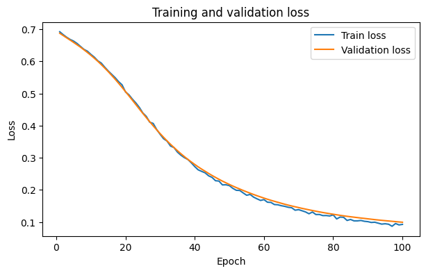
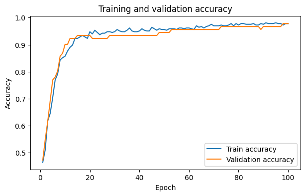
9) Plot training curves

After the training we need to evaluate, how our model performed durning training. Here we have a look how the error that the model predoces behaves over the epochs of the training for the training data and the validation data.

Terminology: Underfitting - the model is too simple to learn the pattern, so performance is poor on both training and validation/test data.
Overfitting - the model fits training data very well but does not generalize, so validation/test performance is worse.

epochs = np.arange(1, num_epochs + 1)

plt.figure(figsize=(7, 4))
plt.plot(epochs, history["train_loss"], label="Train loss")
plt.plot(epochs, history["val_loss"], label="Validation loss")
plt.xlabel("Epoch")
plt.ylabel("Loss")
plt.title("Training and validation loss")
plt.legend()
plt.show()

plt.figure(figsize=(7, 4))
plt.plot(epochs, history["train_acc"], label="Train accuracy")
plt.plot(epochs, history["val_acc"], label="Validation accuracy")
plt.xlabel("Epoch")
plt.ylabel("Accuracy")
plt.title("Training and validation accuracy")
plt.legend()
plt.show()

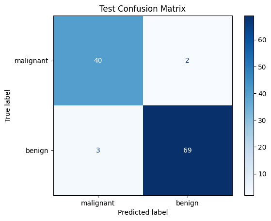
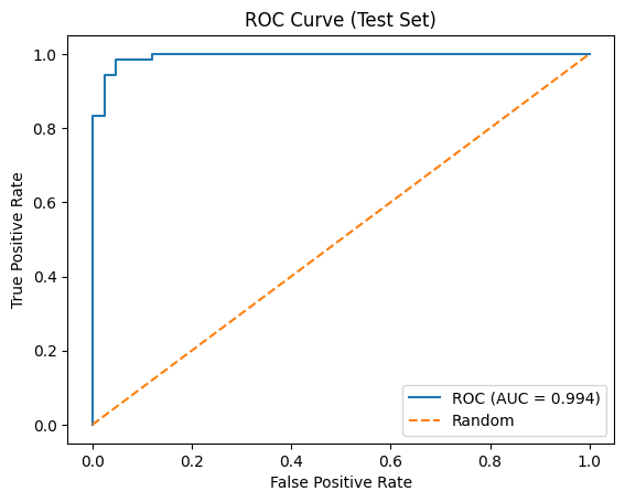
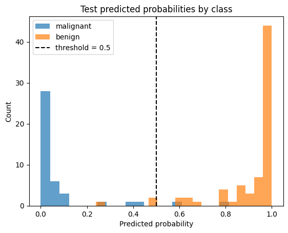
10) Final evaluation on test set

We also need to evaluate how our model will perform on new, unseen data. Therefore, we have the test dataset. We can generate metrics derived from the prediction values of the model and the actual labels of the patients.

test_loss, test_acc, test_probs, test_preds, test_targets = evaluate(
    model, test_loader, criterion, device
)

print(f"Test loss: {test_loss:.4f}")
print(f"Test accuracy: {test_acc:.4f}")

print("\nClassification report:")
print(classification_report(test_targets, test_preds, target_names=data.target_names))

Test loss: 0.1151
Test accuracy: 0.9561

Classification report:
              precision    recall  f1-score   support

   malignant       0.93      0.95      0.94        42
      benign       0.97      0.96      0.97        72

    accuracy                           0.96       114
   macro avg       0.95      0.96      0.95       114
weighted avg       0.96      0.96      0.96       114

cm = confusion_matrix(test_targets, test_preds)
disp = ConfusionMatrixDisplay(confusion_matrix=cm, display_labels=data.target_names)
disp.plot(cmap="Blues", values_format="d")
plt.title("Test Confusion Matrix")
plt.show()

fpr, tpr, thresholds = roc_curve(test_targets.ravel(), test_probs.ravel())
roc_auc = auc(fpr, tpr)

plt.figure()
plt.plot(fpr, tpr, label=f"ROC (AUC = {roc_auc:.3f})")
plt.plot([0, 1], [0, 1], linestyle="--", label="Random")
plt.xlabel("False Positive Rate")
plt.ylabel("True Positive Rate")
plt.title("ROC Curve (Test Set)")
plt.legend()
plt.show()

p = test_probs.ravel()
y = test_targets.ravel()

plt.figure()
plt.hist(p[y == 0], bins=20, alpha=0.7, label=f"{data.target_names[0]}")
plt.hist(p[y == 1], bins=20, alpha=0.7, label=f"{data.target_names[1]}")
plt.axvline(0.5, linestyle="--", label="threshold = 0.5", c='black')
plt.xlabel("Predicted probability")
plt.ylabel("Count")
plt.title("Test predicted probabilities by class")
plt.legend()
plt.show()

Exercise 1: What happens if you change the learning rate ? For example, try out 1e-2, 1e-6, 1e-10.

Exercise 2: Adapt the epochs also in regard to changed learning rates. When do you think your model finishes learning ?

Exercise 3: Change the network architecture. Add or remove linear layers, change dropout rates and activation functions. How does the behaviour of the model change ?

Exercise 4: (Optional) Implement you a 5-fold cross-validation training loop and see check how variable your results are across different splits of the data. (You may ask bob for help.)