Predicting Chronic Heart Failure - Solution#
Spoiler:
This notebook contains a comprehensive step-by-step solution to the exercise.
Try working through the exercise on your own first before looking at this suggested solution.
Clinical Use Case#
Patients admitted with myocardial infarction (MI) are at risk of developing a range of complications, including chronic heart failure (CHF).
Chronic heart failure is a serious condition that can significantly impair quality of life and is associated with increased morbidity and mortality.
Following an acute myocardial infarction, some patients recover without long-term consequences, while others develop progressive cardiac dysfunction leading to heart failure.
Early identification of patients at risk of developing chronic heart failure is challenging, even for experienced clinicians, but highly relevant for optimizing treatment and improving long-term outcomes.
Goal of this analysis:
Build a machine learning model that predicts whether a patient will develop chronic heart failure during hospitalization.
You can download the dataset of myocardial infarction complications from the University of Leicester here: https://figshare.le.ac.uk/ndownloader/files/23581310
About the Dataset#
This dataset contains clinical information about patients admitted with myocardial infarction and was designed to evaluate real-world medical prediction problems.
Variables include:
demographic data
medical history
ECG findings
laboratory values
treatment information
Possible complications are stored in the target variables.
In this notebook, we focus on predicting:
Chronic Heart Failure
Additional information about the dataset, including variable descriptions, can be found here: https://doi.org/10.25392/leicester.data.12045261
Important methodological aspect
The dataset allows prediction at different time points during the hospital stay:
At admission
After 24 hours
After 48 hours
After 72 hours
Depending on the chosen time point, different variables are available.
For this exercise, you must decide on one time point and adapt your feature selection accordingly.
For example:
If you predict at admission, you may only use variables available at admission
Later time points allow more information, but also introduce the risk of data leakage
This reflects a key challenge in clinical machine learning:
Predictions must be based only on information that is available at the time the decision is made.
Potential clinical use:
early identification of patients at risk of chronic heart failure
timely initiation of preventive or therapeutic interventions
improved long-term management and follow-up planning
Your Tasks#
Load and explore the dataset to understand its structure and contents
Decide at which time point you want to predict the ventricular fibrillation (target variable = “FIBR_JELUD”)
Adjust your feature selection accordinglyPrepare the data for machine learning
Train and compare different models (e.g. Logistic Regression, Random Forest, XGB)
Evaluate model performance using appropriate metrics
Interpret your results and reflect on their clinical relevance
# Import bia-bob as a helpful Python & Medical AI expert
from bia_bob import bob
import os

bob.initialize(
    endpoint=os.getenv('ENDPOINT_URL'),
    model="vllm-llama-4-scout-17b-16e-instruct",
    system_prompt=os.getenv('SYSTEM_PROMPT_MEDICAL_AI')
)
%bob Who are you? Just one sentence!
NOTE#
In this notebook we focus on predicting:
Chronic heart failure (ZSN) at the time of admission to the hospital
Therefore, we use all input columns (2-112) except 93, 94, 95, 100, 101, 102, 103, 104, 105.
Step 1: Load and inspect the data#
import pandas as pd
import numpy as np

import matplotlib.pyplot as plt
import seaborn as sns

from sklearn.model_selection import train_test_split
from sklearn.model_selection import GridSearchCV

from sklearn.pipeline import Pipeline
from sklearn.compose import ColumnTransformer

from sklearn.preprocessing import StandardScaler
from sklearn.preprocessing import OneHotEncoder

from sklearn.impute import SimpleImputer

from sklearn.linear_model import LogisticRegression
from sklearn.ensemble import RandomForestClassifier

from xgboost import XGBClassifier

from sklearn.metrics import roc_auc_score
from sklearn.metrics import classification_report
from sklearn.metrics import roc_curve
from sklearn.metrics import confusion_matrix
from sklearn.metrics import RocCurveDisplay

import shap
pd.set_option('display.max_rows', 500)
pd.set_option('display.max_columns', 500)
# load the dataset
df = pd.read_csv('Myocardial_infarction_complications_Database.csv')
df.head()
| ID | AGE | SEX | INF_ANAM | STENOK_AN | FK_STENOK | IBS_POST | IBS_NASL | GB | SIM_GIPERT | DLIT_AG | ZSN_A | nr_11 | nr_01 | nr_02 | nr_03 | nr_04 | nr_07 | nr_08 | np_01 | np_04 | np_05 | np_07 | np_08 | np_09 | np_10 | endocr_01 | endocr_02 | endocr_03 | zab_leg_01 | zab_leg_02 | zab_leg_03 | zab_leg_04 | zab_leg_06 | S_AD_KBRIG | D_AD_KBRIG | S_AD_ORIT | D_AD_ORIT | O_L_POST | K_SH_POST | MP_TP_POST | SVT_POST | GT_POST | FIB_G_POST | ant_im | lat_im | inf_im | post_im | IM_PG_P | ritm_ecg_p_01 | ritm_ecg_p_02 | ritm_ecg_p_04 | ritm_ecg_p_06 | ritm_ecg_p_07 | ritm_ecg_p_08 | n_r_ecg_p_01 | n_r_ecg_p_02 | n_r_ecg_p_03 | n_r_ecg_p_04 | n_r_ecg_p_05 | n_r_ecg_p_06 | n_r_ecg_p_08 | n_r_ecg_p_09 | n_r_ecg_p_10 | n_p_ecg_p_01 | n_p_ecg_p_03 | n_p_ecg_p_04 | n_p_ecg_p_05 | n_p_ecg_p_06 | n_p_ecg_p_07 | n_p_ecg_p_08 | n_p_ecg_p_09 | n_p_ecg_p_10 | n_p_ecg_p_11 | n_p_ecg_p_12 | fibr_ter_01 | fibr_ter_02 | fibr_ter_03 | fibr_ter_05 | fibr_ter_06 | fibr_ter_07 | fibr_ter_08 | GIPO_K | K_BLOOD | GIPER_NA | NA_BLOOD | ALT_BLOOD | AST_BLOOD | KFK_BLOOD | L_BLOOD | ROE | TIME_B_S | R_AB_1_n | R_AB_2_n | R_AB_3_n | NA_KB | NOT_NA_KB | LID_KB | NITR_S | NA_R_1_n | NA_R_2_n | NA_R_3_n | NOT_NA_1_n | NOT_NA_2_n | NOT_NA_3_n | LID_S_n | B_BLOK_S_n | ANT_CA_S_n | GEPAR_S_n | ASP_S_n | TIKL_S_n | TRENT_S_n | FIBR_PREDS | PREDS_TAH | JELUD_TAH | FIBR_JELUD | A_V_BLOK | OTEK_LANC | RAZRIV | DRESSLER | ZSN | REC_IM | P_IM_STEN | LET_IS | |
|---|---|---|---|---|---|---|---|---|---|---|---|---|---|---|---|---|---|---|---|---|---|---|---|---|---|---|---|---|---|---|---|---|---|---|---|---|---|---|---|---|---|---|---|---|---|---|---|---|---|---|---|---|---|---|---|---|---|---|---|---|---|---|---|---|---|---|---|---|---|---|---|---|---|---|---|---|---|---|---|---|---|---|---|---|---|---|---|---|---|---|---|---|---|---|---|---|---|---|---|---|---|---|---|---|---|---|---|---|---|---|---|---|---|---|---|---|---|---|---|---|---|---|---|---|
| 0 | 1 | 77.0 | 1 | 2.0 | 1.0 | 1.0 | 2.0 | NaN | 3.0 | 0.0 | 7.0 | 0.0 | 0.0 | 0.0 | 0.0 | 0.0 | 0.0 | 0.0 | 0.0 | 0.0 | 0.0 | 0.0 | 0.0 | 0.0 | 0.0 | 0.0 | 0.0 | 0.0 | 0.0 | 0.0 | 0.0 | 0.0 | 0.0 | 0.0 | NaN | NaN | 180.0 | 100.0 | 0.0 | 0.0 | 0.0 | 0.0 | 0.0 | 0.0 | 1.0 | 0.0 | 0.0 | 0.0 | 0.0 | 0.0 | 0.0 | 0.0 | 0.0 | 1.0 | 0.0 | 0.0 | 0.0 | 0.0 | 0.0 | 1.0 | 0.0 | 0.0 | 0.0 | 0.0 | 0.0 | 0.0 | 0.0 | 0.0 | 0.0 | 0.0 | 1.0 | 0.0 | 0.0 | 0.0 | 0.0 | 0.0 | 0.0 | 0.0 | 0.0 | 0.0 | 0.0 | 0.0 | 0.0 | 4.7 | 0.0 | 138.0 | NaN | NaN | NaN | 8.0 | 16.0 | 4.0 | 0.0 | 0.0 | 1.0 | NaN | NaN | NaN | 0.0 | 0.0 | 0.0 | 0.0 | 0.0 | 0.0 | 0.0 | 1.0 | 0.0 | 0.0 | 1.0 | 1.0 | 0.0 | 0.0 | 0 | 0 | 0 | 0 | 0 | 0 | 0 | 0 | 0 | 0 | 0 | 0 |
| 1 | 2 | 55.0 | 1 | 1.0 | 0.0 | 0.0 | 0.0 | 0.0 | 0.0 | 0.0 | 0.0 | 0.0 | 0.0 | 0.0 | 0.0 | 0.0 | 0.0 | 0.0 | 0.0 | 0.0 | 0.0 | 0.0 | 0.0 | 0.0 | 0.0 | 0.0 | 0.0 | 0.0 | 0.0 | 0.0 | 0.0 | 0.0 | 0.0 | 0.0 | NaN | NaN | 120.0 | 90.0 | 0.0 | 0.0 | 0.0 | 0.0 | 0.0 | 0.0 | 4.0 | 1.0 | 0.0 | 0.0 | 0.0 | 1.0 | 0.0 | 0.0 | 0.0 | 0.0 | 0.0 | 0.0 | 0.0 | 0.0 | 1.0 | 0.0 | 0.0 | 0.0 | 0.0 | 0.0 | 0.0 | 0.0 | 0.0 | 0.0 | 0.0 | 0.0 | 0.0 | 0.0 | 0.0 | 0.0 | 0.0 | 0.0 | 0.0 | 0.0 | 0.0 | 0.0 | 0.0 | 0.0 | 1.0 | 3.5 | 0.0 | 132.0 | 0.38 | 0.18 | NaN | 7.8 | 3.0 | 2.0 | 0.0 | 0.0 | 0.0 | 1.0 | 0.0 | 1.0 | 0.0 | 0.0 | 0.0 | 0.0 | 1.0 | 0.0 | 0.0 | 1.0 | 0.0 | 1.0 | 1.0 | 1.0 | 0.0 | 1.0 | 0 | 0 | 0 | 0 | 0 | 0 | 0 | 0 | 0 | 0 | 0 | 0 |
| 2 | 3 | 52.0 | 1 | 0.0 | 0.0 | 0.0 | 2.0 | NaN | 2.0 | 0.0 | 2.0 | 0.0 | 0.0 | 0.0 | 0.0 | 0.0 | 0.0 | 0.0 | 0.0 | 0.0 | 0.0 | 0.0 | 0.0 | 0.0 | 0.0 | 0.0 | 0.0 | 0.0 | 0.0 | 0.0 | 0.0 | 0.0 | 0.0 | 0.0 | 150.0 | 100.0 | 180.0 | 100.0 | 0.0 | 0.0 | 0.0 | 0.0 | 0.0 | 0.0 | 4.0 | 1.0 | 0.0 | 0.0 | 0.0 | 1.0 | 0.0 | 0.0 | 0.0 | 0.0 | 0.0 | 0.0 | 0.0 | 1.0 | 0.0 | 0.0 | 0.0 | 0.0 | 0.0 | 0.0 | 0.0 | 0.0 | 0.0 | 0.0 | 0.0 | 0.0 | 0.0 | 0.0 | 0.0 | 0.0 | 0.0 | 0.0 | 0.0 | 0.0 | 0.0 | 0.0 | 0.0 | 0.0 | 0.0 | 4.0 | 0.0 | 132.0 | 0.30 | 0.11 | NaN | 10.8 | NaN | 3.0 | 3.0 | 0.0 | 0.0 | 1.0 | 1.0 | 1.0 | 0.0 | 1.0 | 0.0 | 0.0 | 3.0 | 2.0 | 2.0 | 1.0 | 1.0 | 0.0 | 1.0 | 1.0 | 0.0 | 0.0 | 0 | 0 | 0 | 0 | 0 | 0 | 0 | 0 | 0 | 0 | 0 | 0 |
| 3 | 4 | 68.0 | 0 | 0.0 | 0.0 | 0.0 | 2.0 | NaN | 2.0 | 0.0 | 3.0 | 1.0 | 0.0 | 0.0 | 0.0 | 0.0 | 0.0 | 0.0 | 0.0 | 0.0 | 0.0 | 0.0 | 0.0 | 0.0 | 0.0 | 0.0 | 0.0 | 0.0 | 0.0 | 1.0 | 0.0 | 0.0 | 0.0 | 0.0 | NaN | NaN | 120.0 | 70.0 | 0.0 | 0.0 | 0.0 | 0.0 | 0.0 | 0.0 | 0.0 | 1.0 | 1.0 | 0.0 | 0.0 | 1.0 | 0.0 | 0.0 | 0.0 | 0.0 | 0.0 | 0.0 | 0.0 | 0.0 | 0.0 | 0.0 | 0.0 | 0.0 | 0.0 | 0.0 | 0.0 | 0.0 | 0.0 | 0.0 | 0.0 | 0.0 | 0.0 | 0.0 | 0.0 | 0.0 | 0.0 | 0.0 | 0.0 | 0.0 | 0.0 | 0.0 | 0.0 | 0.0 | 1.0 | 3.9 | 0.0 | 146.0 | 0.75 | 0.37 | NaN | NaN | NaN | 2.0 | 0.0 | 0.0 | 1.0 | NaN | NaN | NaN | 0.0 | 0.0 | 0.0 | 0.0 | 0.0 | 0.0 | 0.0 | 0.0 | 0.0 | 1.0 | 1.0 | 1.0 | 0.0 | 0.0 | 0 | 0 | 0 | 0 | 0 | 0 | 0 | 0 | 1 | 0 | 0 | 0 |
| 4 | 5 | 60.0 | 1 | 0.0 | 0.0 | 0.0 | 2.0 | NaN | 3.0 | 0.0 | 7.0 | 0.0 | 0.0 | 0.0 | 0.0 | 0.0 | 0.0 | 0.0 | 0.0 | 0.0 | 0.0 | 0.0 | 0.0 | 0.0 | 0.0 | 0.0 | 0.0 | 0.0 | 0.0 | 0.0 | 0.0 | 0.0 | 0.0 | 0.0 | 190.0 | 100.0 | 160.0 | 90.0 | 0.0 | 0.0 | 0.0 | 0.0 | 0.0 | 0.0 | 4.0 | 1.0 | 0.0 | 0.0 | 0.0 | 0.0 | 0.0 | 0.0 | 0.0 | 1.0 | 0.0 | 0.0 | 0.0 | 0.0 | 0.0 | 0.0 | 0.0 | 0.0 | 0.0 | 0.0 | 0.0 | 0.0 | 0.0 | 0.0 | 0.0 | 0.0 | 0.0 | 0.0 | 0.0 | 0.0 | 0.0 | 0.0 | 0.0 | 0.0 | 0.0 | 0.0 | 0.0 | 0.0 | 1.0 | 3.5 | 0.0 | 132.0 | 0.45 | 0.22 | NaN | 8.3 | NaN | 9.0 | 0.0 | 0.0 | 0.0 | 0.0 | 0.0 | 0.0 | 0.0 | 0.0 | 0.0 | 0.0 | 0.0 | 0.0 | 0.0 | 0.0 | 0.0 | 1.0 | 0.0 | 1.0 | 0.0 | 1.0 | 0 | 0 | 0 | 0 | 0 | 0 | 0 | 0 | 0 | 0 | 0 | 0 |
# Get dataset size
print("Dataset contains {} rows".format(df.shape[0]))
print("Dataset contains {} columns".format(df.shape[1]))
Dataset contains 1700 rows
Dataset contains 124 columns
# Get summary
df.info()
<class 'pandas.core.frame.DataFrame'>
RangeIndex: 1700 entries, 0 to 1699
Columns: 124 entries, ID to LET_IS
dtypes: float64(110), int64(14)
memory usage: 1.6 MB
# Set patient ID as index (keep column as well)
df = df.set_index("ID", drop=False)
# Define target variable
target = "ZSN"
# Feature Selection (Admission)

# Select predictor columns (2–112)
feature_cols = df.columns[1:112]

# Indices to remove (relative to original df)
drop_idx = [92, 93, 94, 99, 100, 101, 102, 103, 104]

cols_to_remove = df.columns[drop_idx]

# Final feature list
feature_cols = feature_cols.drop(cols_to_remove)

# Keep only relevant columns in df
# IMPORTANT: keep target + selected features
df = df[feature_cols.tolist() + [target]]

# Optional: rename target for clarity
df = df.rename(columns={target: "target"})
# Get new size of the dataset
df.shape
(1700, 103)
df.head()
| AGE | SEX | INF_ANAM | STENOK_AN | FK_STENOK | IBS_POST | IBS_NASL | GB | SIM_GIPERT | DLIT_AG | ZSN_A | nr_11 | nr_01 | nr_02 | nr_03 | nr_04 | nr_07 | nr_08 | np_01 | np_04 | np_05 | np_07 | np_08 | np_09 | np_10 | endocr_01 | endocr_02 | endocr_03 | zab_leg_01 | zab_leg_02 | zab_leg_03 | zab_leg_04 | zab_leg_06 | S_AD_KBRIG | D_AD_KBRIG | S_AD_ORIT | D_AD_ORIT | O_L_POST | K_SH_POST | MP_TP_POST | SVT_POST | GT_POST | FIB_G_POST | ant_im | lat_im | inf_im | post_im | IM_PG_P | ritm_ecg_p_01 | ritm_ecg_p_02 | ritm_ecg_p_04 | ritm_ecg_p_06 | ritm_ecg_p_07 | ritm_ecg_p_08 | n_r_ecg_p_01 | n_r_ecg_p_02 | n_r_ecg_p_03 | n_r_ecg_p_04 | n_r_ecg_p_05 | n_r_ecg_p_06 | n_r_ecg_p_08 | n_r_ecg_p_09 | n_r_ecg_p_10 | n_p_ecg_p_01 | n_p_ecg_p_03 | n_p_ecg_p_04 | n_p_ecg_p_05 | n_p_ecg_p_06 | n_p_ecg_p_07 | n_p_ecg_p_08 | n_p_ecg_p_09 | n_p_ecg_p_10 | n_p_ecg_p_11 | n_p_ecg_p_12 | fibr_ter_01 | fibr_ter_02 | fibr_ter_03 | fibr_ter_05 | fibr_ter_06 | fibr_ter_07 | fibr_ter_08 | GIPO_K | K_BLOOD | GIPER_NA | NA_BLOOD | ALT_BLOOD | AST_BLOOD | KFK_BLOOD | L_BLOOD | ROE | TIME_B_S | NA_KB | NOT_NA_KB | LID_KB | NITR_S | LID_S_n | B_BLOK_S_n | ANT_CA_S_n | GEPAR_S_n | ASP_S_n | TIKL_S_n | TRENT_S_n | target | |
|---|---|---|---|---|---|---|---|---|---|---|---|---|---|---|---|---|---|---|---|---|---|---|---|---|---|---|---|---|---|---|---|---|---|---|---|---|---|---|---|---|---|---|---|---|---|---|---|---|---|---|---|---|---|---|---|---|---|---|---|---|---|---|---|---|---|---|---|---|---|---|---|---|---|---|---|---|---|---|---|---|---|---|---|---|---|---|---|---|---|---|---|---|---|---|---|---|---|---|---|---|---|---|---|
| ID | |||||||||||||||||||||||||||||||||||||||||||||||||||||||||||||||||||||||||||||||||||||||||||||||||||||||
| 1 | 77.0 | 1 | 2.0 | 1.0 | 1.0 | 2.0 | NaN | 3.0 | 0.0 | 7.0 | 0.0 | 0.0 | 0.0 | 0.0 | 0.0 | 0.0 | 0.0 | 0.0 | 0.0 | 0.0 | 0.0 | 0.0 | 0.0 | 0.0 | 0.0 | 0.0 | 0.0 | 0.0 | 0.0 | 0.0 | 0.0 | 0.0 | 0.0 | NaN | NaN | 180.0 | 100.0 | 0.0 | 0.0 | 0.0 | 0.0 | 0.0 | 0.0 | 1.0 | 0.0 | 0.0 | 0.0 | 0.0 | 0.0 | 0.0 | 0.0 | 0.0 | 1.0 | 0.0 | 0.0 | 0.0 | 0.0 | 0.0 | 1.0 | 0.0 | 0.0 | 0.0 | 0.0 | 0.0 | 0.0 | 0.0 | 0.0 | 0.0 | 0.0 | 1.0 | 0.0 | 0.0 | 0.0 | 0.0 | 0.0 | 0.0 | 0.0 | 0.0 | 0.0 | 0.0 | 0.0 | 0.0 | 4.7 | 0.0 | 138.0 | NaN | NaN | NaN | 8.0 | 16.0 | 4.0 | NaN | NaN | NaN | 0.0 | 1.0 | 0.0 | 0.0 | 1.0 | 1.0 | 0.0 | 0.0 | 0 |
| 2 | 55.0 | 1 | 1.0 | 0.0 | 0.0 | 0.0 | 0.0 | 0.0 | 0.0 | 0.0 | 0.0 | 0.0 | 0.0 | 0.0 | 0.0 | 0.0 | 0.0 | 0.0 | 0.0 | 0.0 | 0.0 | 0.0 | 0.0 | 0.0 | 0.0 | 0.0 | 0.0 | 0.0 | 0.0 | 0.0 | 0.0 | 0.0 | 0.0 | NaN | NaN | 120.0 | 90.0 | 0.0 | 0.0 | 0.0 | 0.0 | 0.0 | 0.0 | 4.0 | 1.0 | 0.0 | 0.0 | 0.0 | 1.0 | 0.0 | 0.0 | 0.0 | 0.0 | 0.0 | 0.0 | 0.0 | 0.0 | 1.0 | 0.0 | 0.0 | 0.0 | 0.0 | 0.0 | 0.0 | 0.0 | 0.0 | 0.0 | 0.0 | 0.0 | 0.0 | 0.0 | 0.0 | 0.0 | 0.0 | 0.0 | 0.0 | 0.0 | 0.0 | 0.0 | 0.0 | 0.0 | 1.0 | 3.5 | 0.0 | 132.0 | 0.38 | 0.18 | NaN | 7.8 | 3.0 | 2.0 | 1.0 | 0.0 | 1.0 | 0.0 | 1.0 | 0.0 | 1.0 | 1.0 | 1.0 | 0.0 | 1.0 | 0 |
| 3 | 52.0 | 1 | 0.0 | 0.0 | 0.0 | 2.0 | NaN | 2.0 | 0.0 | 2.0 | 0.0 | 0.0 | 0.0 | 0.0 | 0.0 | 0.0 | 0.0 | 0.0 | 0.0 | 0.0 | 0.0 | 0.0 | 0.0 | 0.0 | 0.0 | 0.0 | 0.0 | 0.0 | 0.0 | 0.0 | 0.0 | 0.0 | 0.0 | 150.0 | 100.0 | 180.0 | 100.0 | 0.0 | 0.0 | 0.0 | 0.0 | 0.0 | 0.0 | 4.0 | 1.0 | 0.0 | 0.0 | 0.0 | 1.0 | 0.0 | 0.0 | 0.0 | 0.0 | 0.0 | 0.0 | 0.0 | 1.0 | 0.0 | 0.0 | 0.0 | 0.0 | 0.0 | 0.0 | 0.0 | 0.0 | 0.0 | 0.0 | 0.0 | 0.0 | 0.0 | 0.0 | 0.0 | 0.0 | 0.0 | 0.0 | 0.0 | 0.0 | 0.0 | 0.0 | 0.0 | 0.0 | 0.0 | 4.0 | 0.0 | 132.0 | 0.30 | 0.11 | NaN | 10.8 | NaN | 3.0 | 1.0 | 1.0 | 1.0 | 0.0 | 1.0 | 1.0 | 0.0 | 1.0 | 1.0 | 0.0 | 0.0 | 0 |
| 4 | 68.0 | 0 | 0.0 | 0.0 | 0.0 | 2.0 | NaN | 2.0 | 0.0 | 3.0 | 1.0 | 0.0 | 0.0 | 0.0 | 0.0 | 0.0 | 0.0 | 0.0 | 0.0 | 0.0 | 0.0 | 0.0 | 0.0 | 0.0 | 0.0 | 0.0 | 0.0 | 0.0 | 1.0 | 0.0 | 0.0 | 0.0 | 0.0 | NaN | NaN | 120.0 | 70.0 | 0.0 | 0.0 | 0.0 | 0.0 | 0.0 | 0.0 | 0.0 | 1.0 | 1.0 | 0.0 | 0.0 | 1.0 | 0.0 | 0.0 | 0.0 | 0.0 | 0.0 | 0.0 | 0.0 | 0.0 | 0.0 | 0.0 | 0.0 | 0.0 | 0.0 | 0.0 | 0.0 | 0.0 | 0.0 | 0.0 | 0.0 | 0.0 | 0.0 | 0.0 | 0.0 | 0.0 | 0.0 | 0.0 | 0.0 | 0.0 | 0.0 | 0.0 | 0.0 | 0.0 | 1.0 | 3.9 | 0.0 | 146.0 | 0.75 | 0.37 | NaN | NaN | NaN | 2.0 | NaN | NaN | NaN | 0.0 | 0.0 | 0.0 | 1.0 | 1.0 | 1.0 | 0.0 | 0.0 | 1 |
| 5 | 60.0 | 1 | 0.0 | 0.0 | 0.0 | 2.0 | NaN | 3.0 | 0.0 | 7.0 | 0.0 | 0.0 | 0.0 | 0.0 | 0.0 | 0.0 | 0.0 | 0.0 | 0.0 | 0.0 | 0.0 | 0.0 | 0.0 | 0.0 | 0.0 | 0.0 | 0.0 | 0.0 | 0.0 | 0.0 | 0.0 | 0.0 | 0.0 | 190.0 | 100.0 | 160.0 | 90.0 | 0.0 | 0.0 | 0.0 | 0.0 | 0.0 | 0.0 | 4.0 | 1.0 | 0.0 | 0.0 | 0.0 | 0.0 | 0.0 | 0.0 | 0.0 | 1.0 | 0.0 | 0.0 | 0.0 | 0.0 | 0.0 | 0.0 | 0.0 | 0.0 | 0.0 | 0.0 | 0.0 | 0.0 | 0.0 | 0.0 | 0.0 | 0.0 | 0.0 | 0.0 | 0.0 | 0.0 | 0.0 | 0.0 | 0.0 | 0.0 | 0.0 | 0.0 | 0.0 | 0.0 | 1.0 | 3.5 | 0.0 | 132.0 | 0.45 | 0.22 | NaN | 8.3 | NaN | 9.0 | 0.0 | 0.0 | 0.0 | 0.0 | 0.0 | 0.0 | 1.0 | 0.0 | 1.0 | 0.0 | 1.0 | 0 |
# Detect feature types

binary_features = []
categorical_features = []
continuous_features = []

for col in feature_cols:

    n_unique = df[col].nunique(dropna=True)

    # Binary: exactly 2 unique values
    if n_unique == 2:
        binary_features.append(col)

    # Categorical: few unique values (but not binary)
    elif n_unique < 10:
        categorical_features.append(col)

    # Continuous: many unique values
    else:
        continuous_features.append(col)
# Assign data types
df[binary_features] = df[binary_features].astype("category")
df[categorical_features] = df[categorical_features].astype("category")
# Overview of
print("Binary features:", len(binary_features))
print("Categorical features:", len(categorical_features))
print("Continuous features:", len(continuous_features))
Binary features: 78
Categorical features: 13
Continuous features: 11
df.dtypes.value_counts()
category    77
float64     11
category     6
category     2
category     1
category     1
category     1
category     1
category     1
category     1
int64        1
Name: count, dtype: int64
# Summary statistics for numeric columns
df.describe(include=['int', 'float']).T
| count | mean | std | min | 25% | 50% | 75% | max | |
|---|---|---|---|---|---|---|---|---|
| AGE | 1692.0 | 61.856974 | 11.259936 | 26.00 | 54.00 | 63.00 | 70.00 | 92.00 |
| S_AD_KBRIG | 624.0 | 136.907051 | 34.997835 | 0.00 | 120.00 | 140.00 | 160.00 | 260.00 |
| D_AD_KBRIG | 624.0 | 81.394231 | 19.745045 | 0.00 | 70.00 | 80.00 | 90.00 | 190.00 |
| S_AD_ORIT | 1433.0 | 134.588276 | 31.348388 | 0.00 | 120.00 | 130.00 | 150.00 | 260.00 |
| D_AD_ORIT | 1433.0 | 82.749477 | 18.321063 | 0.00 | 80.00 | 80.00 | 90.00 | 190.00 |
| K_BLOOD | 1329.0 | 4.191422 | 0.754076 | 2.30 | 3.70 | 4.10 | 4.60 | 8.20 |
| NA_BLOOD | 1325.0 | 136.550943 | 6.512120 | 117.00 | 133.00 | 136.00 | 140.00 | 169.00 |
| ALT_BLOOD | 1416.0 | 0.481455 | 0.387261 | 0.03 | 0.23 | 0.38 | 0.61 | 3.00 |
| AST_BLOOD | 1415.0 | 0.263717 | 0.201802 | 0.04 | 0.15 | 0.22 | 0.33 | 2.15 |
| L_BLOOD | 1575.0 | 8.782914 | 3.400557 | 2.00 | 6.40 | 8.00 | 10.45 | 27.90 |
| ROE | 1497.0 | 13.444890 | 11.296316 | 1.00 | 5.00 | 10.00 | 18.00 | 140.00 |
| target | 1700.0 | 0.231765 | 0.422084 | 0.00 | 0.00 | 0.00 | 0.00 | 1.00 |
# Summary statistics for categorical columns
df.describe(include="category").T
| count | unique | top | freq | |
|---|---|---|---|---|
| SEX | 1700.0 | 2.0 | 1.0 | 1065.0 |
| INF_ANAM | 1696.0 | 4.0 | 0.0 | 1060.0 |
| STENOK_AN | 1594.0 | 7.0 | 0.0 | 661.0 |
| FK_STENOK | 1627.0 | 5.0 | 2.0 | 854.0 |
| IBS_POST | 1649.0 | 3.0 | 2.0 | 683.0 |
| IBS_NASL | 72.0 | 2.0 | 0.0 | 45.0 |
| GB | 1691.0 | 4.0 | 2.0 | 880.0 |
| SIM_GIPERT | 1692.0 | 2.0 | 0.0 | 1635.0 |
| DLIT_AG | 1452.0 | 8.0 | 0.0 | 551.0 |
| ZSN_A | 1646.0 | 5.0 | 0.0 | 1468.0 |
| nr_11 | 1679.0 | 2.0 | 0.0 | 1637.0 |
| nr_01 | 1679.0 | 2.0 | 0.0 | 1675.0 |
| nr_02 | 1679.0 | 2.0 | 0.0 | 1660.0 |
| nr_03 | 1679.0 | 2.0 | 0.0 | 1644.0 |
| nr_04 | 1679.0 | 2.0 | 0.0 | 1650.0 |
| nr_07 | 1679.0 | 2.0 | 0.0 | 1678.0 |
| nr_08 | 1679.0 | 2.0 | 0.0 | 1675.0 |
| np_01 | 1682.0 | 2.0 | 0.0 | 1680.0 |
| np_04 | 1682.0 | 2.0 | 0.0 | 1679.0 |
| np_05 | 1682.0 | 2.0 | 0.0 | 1671.0 |
| np_07 | 1682.0 | 2.0 | 0.0 | 1681.0 |
| np_08 | 1682.0 | 2.0 | 0.0 | 1676.0 |
| np_09 | 1682.0 | 2.0 | 0.0 | 1680.0 |
| np_10 | 1682.0 | 2.0 | 0.0 | 1679.0 |
| endocr_01 | 1689.0 | 2.0 | 0.0 | 1461.0 |
| endocr_02 | 1690.0 | 2.0 | 0.0 | 1648.0 |
| endocr_03 | 1690.0 | 2.0 | 0.0 | 1677.0 |
| zab_leg_01 | 1693.0 | 2.0 | 0.0 | 1559.0 |
| zab_leg_02 | 1693.0 | 2.0 | 0.0 | 1572.0 |
| zab_leg_03 | 1693.0 | 2.0 | 0.0 | 1656.0 |
| zab_leg_04 | 1693.0 | 2.0 | 0.0 | 1684.0 |
| zab_leg_06 | 1693.0 | 2.0 | 0.0 | 1671.0 |
| O_L_POST | 1688.0 | 2.0 | 0.0 | 1578.0 |
| K_SH_POST | 1685.0 | 2.0 | 0.0 | 1639.0 |
| MP_TP_POST | 1686.0 | 2.0 | 0.0 | 1572.0 |
| SVT_POST | 1688.0 | 2.0 | 0.0 | 1680.0 |
| GT_POST | 1688.0 | 2.0 | 0.0 | 1680.0 |
| FIB_G_POST | 1688.0 | 2.0 | 0.0 | 1673.0 |
| ant_im | 1617.0 | 5.0 | 0.0 | 660.0 |
| lat_im | 1620.0 | 5.0 | 1.0 | 838.0 |
| inf_im | 1620.0 | 5.0 | 0.0 | 937.0 |
| post_im | 1628.0 | 5.0 | 0.0 | 1370.0 |
| IM_PG_P | 1699.0 | 2.0 | 0.0 | 1649.0 |
| ritm_ecg_p_01 | 1548.0 | 2.0 | 1.0 | 1029.0 |
| ritm_ecg_p_02 | 1548.0 | 2.0 | 0.0 | 1453.0 |
| ritm_ecg_p_04 | 1548.0 | 2.0 | 0.0 | 1525.0 |
| ritm_ecg_p_06 | 1548.0 | 2.0 | 0.0 | 1547.0 |
| ritm_ecg_p_07 | 1548.0 | 2.0 | 0.0 | 1195.0 |
| ritm_ecg_p_08 | 1548.0 | 2.0 | 0.0 | 1502.0 |
| n_r_ecg_p_01 | 1585.0 | 2.0 | 0.0 | 1527.0 |
| n_r_ecg_p_02 | 1585.0 | 2.0 | 0.0 | 1577.0 |
| n_r_ecg_p_03 | 1585.0 | 2.0 | 0.0 | 1381.0 |
| n_r_ecg_p_04 | 1585.0 | 2.0 | 0.0 | 1516.0 |
| n_r_ecg_p_05 | 1585.0 | 2.0 | 0.0 | 1515.0 |
| n_r_ecg_p_06 | 1585.0 | 2.0 | 0.0 | 1553.0 |
| n_r_ecg_p_08 | 1585.0 | 2.0 | 0.0 | 1581.0 |
| n_r_ecg_p_09 | 1585.0 | 2.0 | 0.0 | 1583.0 |
| n_r_ecg_p_10 | 1585.0 | 2.0 | 0.0 | 1583.0 |
| n_p_ecg_p_01 | 1585.0 | 2.0 | 0.0 | 1583.0 |
| n_p_ecg_p_03 | 1585.0 | 2.0 | 0.0 | 1553.0 |
| n_p_ecg_p_04 | 1585.0 | 2.0 | 0.0 | 1580.0 |
| n_p_ecg_p_05 | 1585.0 | 2.0 | 0.0 | 1583.0 |
| n_p_ecg_p_06 | 1585.0 | 2.0 | 0.0 | 1558.0 |
| n_p_ecg_p_07 | 1585.0 | 2.0 | 0.0 | 1483.0 |
| n_p_ecg_p_08 | 1585.0 | 2.0 | 0.0 | 1578.0 |
| n_p_ecg_p_09 | 1585.0 | 2.0 | 0.0 | 1575.0 |
| n_p_ecg_p_10 | 1585.0 | 2.0 | 0.0 | 1551.0 |
| n_p_ecg_p_11 | 1585.0 | 2.0 | 0.0 | 1557.0 |
| n_p_ecg_p_12 | 1585.0 | 2.0 | 0.0 | 1507.0 |
| fibr_ter_01 | 1690.0 | 2.0 | 0.0 | 1677.0 |
| fibr_ter_02 | 1690.0 | 2.0 | 0.0 | 1674.0 |
| fibr_ter_03 | 1690.0 | 2.0 | 0.0 | 1622.0 |
| fibr_ter_05 | 1690.0 | 2.0 | 0.0 | 1686.0 |
| fibr_ter_06 | 1690.0 | 2.0 | 0.0 | 1681.0 |
| fibr_ter_07 | 1690.0 | 2.0 | 0.0 | 1684.0 |
| fibr_ter_08 | 1690.0 | 2.0 | 0.0 | 1688.0 |
| GIPO_K | 1331.0 | 2.0 | 0.0 | 797.0 |
| GIPER_NA | 1325.0 | 2.0 | 0.0 | 1295.0 |
| KFK_BLOOD | 4.0 | 4.0 | 1.2 | 1.0 |
| TIME_B_S | 1574.0 | 9.0 | 2.0 | 360.0 |
| NA_KB | 1043.0 | 2.0 | 1.0 | 618.0 |
| NOT_NA_KB | 1014.0 | 2.0 | 1.0 | 701.0 |
| LID_KB | 1023.0 | 2.0 | 0.0 | 627.0 |
| NITR_S | 1691.0 | 2.0 | 0.0 | 1496.0 |
| LID_S_n | 1690.0 | 2.0 | 0.0 | 1211.0 |
| B_BLOK_S_n | 1689.0 | 2.0 | 0.0 | 1474.0 |
| ANT_CA_S_n | 1687.0 | 2.0 | 1.0 | 1125.0 |
| GEPAR_S_n | 1683.0 | 2.0 | 1.0 | 1203.0 |
| ASP_S_n | 1683.0 | 2.0 | 1.0 | 1252.0 |
| TIKL_S_n | 1684.0 | 2.0 | 0.0 | 1654.0 |
| TRENT_S_n | 1684.0 | 2.0 | 0.0 | 1343.0 |
Step 2: Exploratory Data Analysis (EDA)#
Before training machine learning models, it is important to understand the structure of the dataset.
In this section we explore:
distribution of target variable
missing values
class imbalance
df['target'].value_counts()
target
0    1306
1     394
Name: count, dtype: int64
sns.countplot(x='target', data=df)
plt.title("Distribution of Chronic Heart Failure")
plt.show()
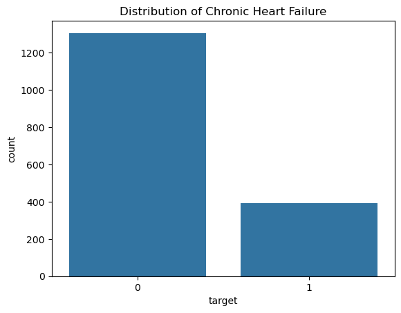
-> Class Imbalance
Chronic Heart Failure is a rare event in this dataset.
This creates a class imbalance problem, meaning that most patients belong to the negative class.
This can lead to biased models that simply predict the majority class.
To address this issue we will later use:
class weights
adjusted thresholds
ROC-AUC evaluation
Visualization of prediction variables#
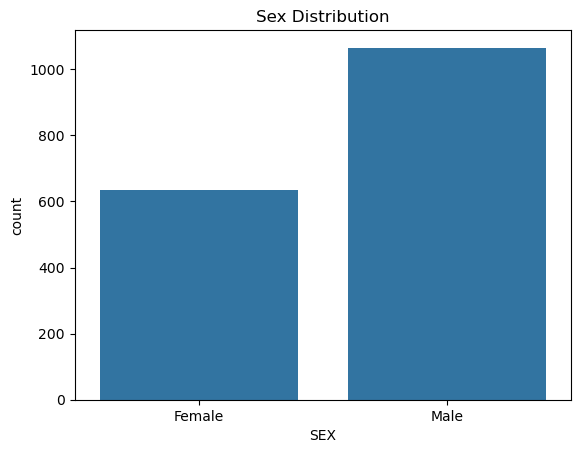
# NOTE: 0 - female, 1 - male
sns.countplot(x=df['SEX'].map({0: "Female", 1: "Male"}), data=df)
plt.title("Sex Distribution")
plt.show()
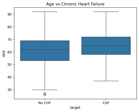
sns.boxplot(x=df['target'].map({0: "No CHF", 1: "CHF"}), y="AGE", data=df)
plt.title("Age vs Chronic Heart Failure")
plt.show()
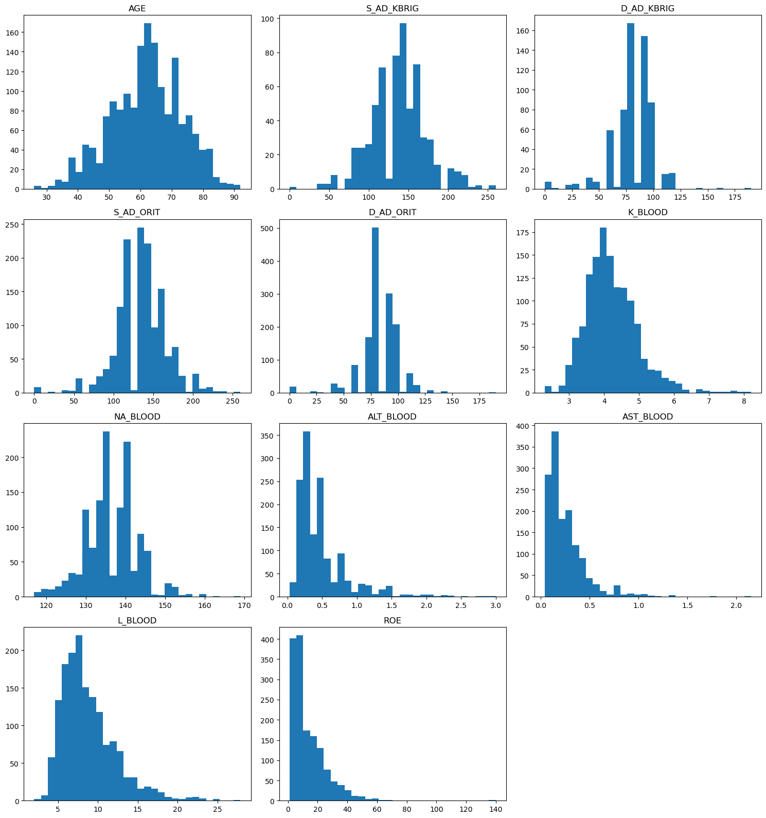
import matplotlib.pyplot as plt
import math

# number of plots
n_features = len(continuous_features)

# define grid size
n_cols = 3
n_rows = math.ceil(n_features / n_cols)

# create figure
fig, axes = plt.subplots(n_rows, n_cols, figsize=(15, 4 * n_rows))

# flatten axes (important!)
axes = axes.flatten()

# plot each feature
for i, col in enumerate(continuous_features):

    axes[i].hist(df[col].dropna(), bins=30)
    axes[i].set_title(col)

# remove empty plots
for j in range(i + 1, len(axes)):
    fig.delaxes(axes[j])

plt.tight_layout()
plt.show()
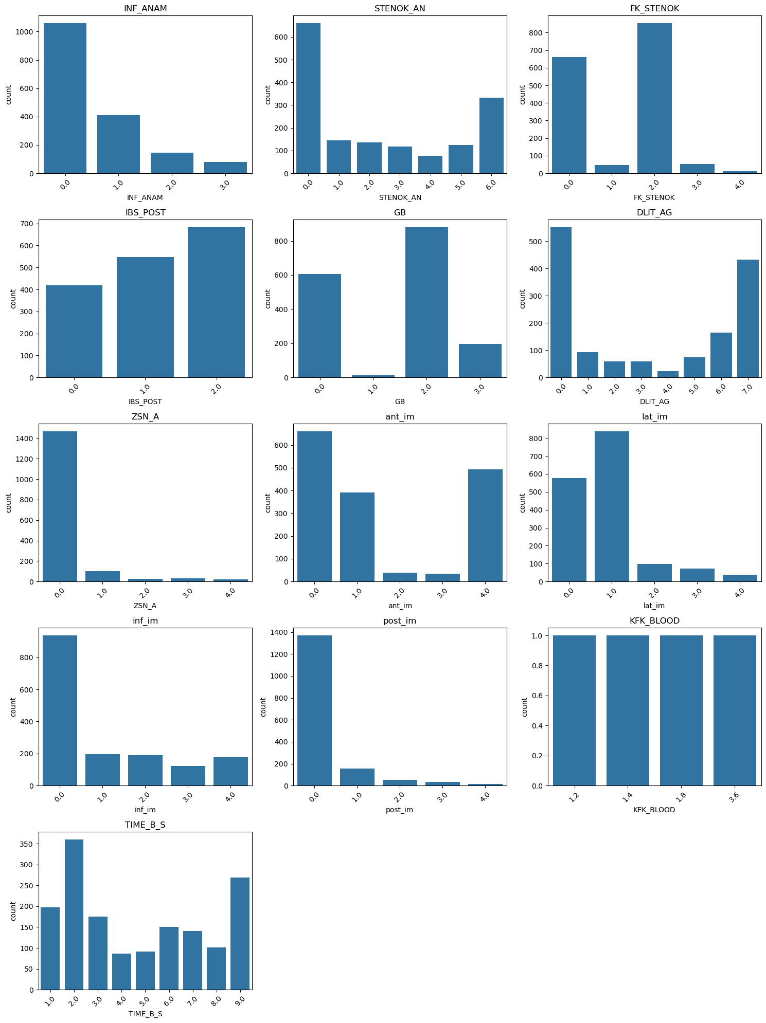
# number of plots
n_features = len(categorical_features)

# grid size
n_cols = 3
n_rows = math.ceil(n_features / n_cols)

# create figure
fig, axes = plt.subplots(n_rows, n_cols, figsize=(15, 4 * n_rows))

axes = axes.flatten()

# plot each categorical feature
for i, col in enumerate(categorical_features):

    sns.countplot(x=df[col], ax=axes[i])
    axes[i].set_title(col)
    axes[i].tick_params(axis='x', rotation=45)

# remove empty plots
for j in range(i + 1, len(axes)):
    fig.delaxes(axes[j])

plt.tight_layout()
plt.show()
Check for missing values#
# Get table with missing value counts and percentage for each feature
missing_summary = pd.DataFrame({
    "missing_count": df.isna().sum(),
    "missing_percent": df.isna().mean() * 100
})

missing_summary = missing_summary.sort_values(
    "missing_percent", ascending=False
)

missing_summary.head(25)
| missing_count | missing_percent | |
|---|---|---|
| KFK_BLOOD | 1696 | 99.764706 |
| IBS_NASL | 1628 | 95.764706 |
| D_AD_KBRIG | 1076 | 63.294118 |
| S_AD_KBRIG | 1076 | 63.294118 |
| NOT_NA_KB | 686 | 40.352941 |
| LID_KB | 677 | 39.823529 |
| NA_KB | 657 | 38.647059 |
| NA_BLOOD | 375 | 22.058824 |
| GIPER_NA | 375 | 22.058824 |
| K_BLOOD | 371 | 21.823529 |
| GIPO_K | 369 | 21.705882 |
| AST_BLOOD | 285 | 16.764706 |
| ALT_BLOOD | 284 | 16.705882 |
| D_AD_ORIT | 267 | 15.705882 |
| S_AD_ORIT | 267 | 15.705882 |
| DLIT_AG | 248 | 14.588235 |
| ROE | 203 | 11.941176 |
| ritm_ecg_p_08 | 152 | 8.941176 |
| ritm_ecg_p_07 | 152 | 8.941176 |
| ritm_ecg_p_04 | 152 | 8.941176 |
| ritm_ecg_p_02 | 152 | 8.941176 |
| ritm_ecg_p_01 | 152 | 8.941176 |
| ritm_ecg_p_06 | 152 | 8.941176 |
| TIME_B_S | 126 | 7.411765 |
| L_BLOOD | 125 | 7.352941 |
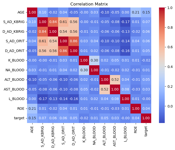
Correlation Analysis#
We inspect correlations between continuous variables.
Highly correlated variables often measure similar physiological processes.
Tree-based models such as Random Forest and XGBoost can handle correlated predictors relatively well, therefore we do not automatically remove them.
# Calculate correlation matrix for numerical features
corr_matrix = df.select_dtypes(include=[np.number]).corr()

# Show correlation table
corr_matrix
| AGE | S_AD_KBRIG | D_AD_KBRIG | S_AD_ORIT | D_AD_ORIT | K_BLOOD | NA_BLOOD | ALT_BLOOD | AST_BLOOD | L_BLOOD | ROE | target | |
|---|---|---|---|---|---|---|---|---|---|---|---|---|
| AGE | 1.000000 | 0.095658 | -0.022013 | 0.043821 | -0.049489 | -0.002999 | 0.031139 | -0.104688 | -0.053533 | 0.003120 | 0.214393 | 0.146107 |
| S_AD_KBRIG | 0.095658 | 1.000000 | 0.844144 | 0.611365 | 0.555501 | -0.004314 | -0.008899 | -0.045470 | -0.083252 | -0.172723 | 0.005249 | 0.072490 |
| D_AD_KBRIG | -0.022013 | 0.844144 | 1.000000 | 0.543048 | 0.555960 | -0.011671 | 0.012838 | -0.056683 | -0.057641 | -0.125900 | -0.022010 | 0.059376 |
| S_AD_ORIT | 0.043821 | 0.611365 | 0.543048 | 1.000000 | 0.861266 | 0.030007 | 0.042669 | -0.102709 | -0.103231 | -0.144040 | 0.040766 | 0.062360 |
| D_AD_ORIT | -0.049489 | 0.555501 | 0.555960 | 0.861266 | 1.000000 | 0.011964 | 0.020672 | -0.059277 | -0.075661 | -0.155752 | 0.011588 | 0.052345 |
| K_BLOOD | -0.002999 | -0.004314 | -0.011671 | 0.030007 | 0.011964 | 1.000000 | 0.300430 | 0.023802 | 0.051519 | 0.012584 | 0.009055 | -0.024080 |
| NA_BLOOD | 0.031139 | -0.008899 | 0.012838 | 0.042669 | 0.020672 | 0.300430 | 1.000000 | -0.005731 | -0.022231 | 0.015816 | -0.013838 | 0.012107 |
| ALT_BLOOD | -0.104688 | -0.045470 | -0.056683 | -0.102709 | -0.059277 | 0.023802 | -0.005731 | 1.000000 | 0.519449 | 0.044393 | -0.007868 | 0.053766 |
| AST_BLOOD | -0.053533 | -0.083252 | -0.057641 | -0.103231 | -0.075661 | 0.051519 | -0.022231 | 0.519449 | 1.000000 | 0.077660 | -0.030673 | 0.032433 |
| L_BLOOD | 0.003120 | -0.172723 | -0.125900 | -0.144040 | -0.155752 | 0.012584 | 0.015816 | 0.044393 | 0.077660 | 1.000000 | 0.005169 | -0.004620 |
| ROE | 0.214393 | 0.005249 | -0.022010 | 0.040766 | 0.011588 | 0.009055 | -0.013838 | -0.007868 | -0.030673 | 0.005169 | 1.000000 | 0.041057 |
| target | 0.146107 | 0.072490 | 0.059376 | 0.062360 | 0.052345 | -0.024080 | 0.012107 | 0.053766 | 0.032433 | -0.004620 | 0.041057 | 1.000000 |
plt.figure(figsize=(8,6))

sns.heatmap(
    corr_matrix,
    annot=True,
    cmap="coolwarm",
    fmt=".2f"
)

plt.title("Correlation Matrix")
plt.show()
Step 3: Feature preprocessing#
Before training machine learning models we need to define which variables should be used as predictors.
The dataset contains more than 100 potential input variables.
However, not all variables are suitable for the prediction of .
We apply three feature selection steps:
Remove identifiers and target variables
Remove variables with excessive missing values
Inspect correlations between continuous variables
Important note:
Tree-based models such as Random Forest and XGBoost are generally robust to correlated predictors, therefore we usually do not automatically remove correlated features unless they are redundant.
Handling Missing Data#
Clinical datasets often contain missing values because:
laboratory tests may not be performed
documentation may be incomplete
measurements may not be available at admission
Therefore, we apply different strategies depending on the variable type:
All variables: Removed if more than 30% of values are missing
missing_percent = df.isna().mean()

# Keep continuous variables with <= 30% missing
continuous_keep = [
    col for col in continuous_features
    if missing_percent[col] <= 0.3
]

# Keep categorical/binary only if no missing values
categorical_keep = [
    col for col in categorical_features
    if missing_percent[col] <= 0.3
]

binary_keep = [
    col for col in binary_features
    if missing_percent[col] <= 0.3
]

# Combine selected features
selected_features = continuous_keep + categorical_keep + binary_keep + ["target"]
df = df[selected_features]
print("After removing binary and categorical features with missing values and continuous features with more than 30% missing values, there are {} features left.".format(len(selected_features) - 1))
After removing binary and categorical features with missing values and continuous features with more than 30% missing values, there are 95 features left.
# Split features and target
X = df.drop(columns="target")
y = df["target"]
Train-Test Split#
To evaluate the model properly we split the dataset into:
training data – used to train the models
test data – used to evaluate performance
We use stratified sampling to preserve the class distribution.
X_train, X_test, y_train, y_test = train_test_split(
    X, y,
    test_size=0.2,
    stratify=y,
    random_state=42
)
Preprocessing pipeline#
Data imputation
Standardization
# Continuous features
continuous_pipeline = Pipeline([
    ("imputer", SimpleImputer(strategy="median")),   # fill missing values
    ("scaler", StandardScaler())                     # normalize values
])

# Categorical + Binary features
categorical_pipeline = Pipeline([
    ("imputer", SimpleImputer(strategy="most_frequent"))  # fill missing values
])
# Combine both pipelines
preprocessor = ColumnTransformer([
    ("num", continuous_pipeline, continuous_keep),
    ("cat", categorical_pipeline, categorical_keep + binary_keep)
])
Encoding of categorical features is not necessary for this dataset, because all features are already encoded.
Step 4: Modeling#
We compare three different machine learning algorithms:
Logistic Regression
simple baseline model
interpretable
Random Forest
ensemble of decision trees
captures non-linear relationships
XGBoost
gradient boosting algorithm
often performs very well on tabular data
logreg_pipeline = Pipeline([
    ("preprocessing", preprocessor),
    ("model", LogisticRegression(max_iter=2000, class_weight="balanced"))
])

rf_pipeline = Pipeline([
    ("preprocessing", preprocessor),
    ("model", RandomForestClassifier(class_weight="balanced"))
])

xgb_pipeline = Pipeline([
    ("preprocessing", preprocessor),
    ("model", XGBClassifier(
        eval_metric="logloss",
        scale_pos_weight=scale_pos_weight
    ))
])
Hyperparameter Tuning#
Machine learning models have parameters that must be chosen before training.
logreg_grid = {
"model__C":[0.01,0.1,1,10]
}
rf_grid = {

"model__n_estimators":[100,300],
"model__max_depth":[5,10,None],
"model__min_samples_split":[2,5]

}
xgb_grid = {

"model__n_estimators":[100,300],
"model__max_depth":[3,6],
"model__learning_rate":[0.01,0.1]

}
print("Columns in X:")
print(X.columns.tolist())
Columns in X:
['AGE', 'S_AD_ORIT', 'D_AD_ORIT', 'K_BLOOD', 'NA_BLOOD', 'ALT_BLOOD', 'AST_BLOOD', 'L_BLOOD', 'ROE', 'INF_ANAM', 'STENOK_AN', 'FK_STENOK', 'IBS_POST', 'GB', 'DLIT_AG', 'ZSN_A', 'ant_im', 'lat_im', 'inf_im', 'post_im', 'TIME_B_S', 'SEX', 'SIM_GIPERT', 'nr_11', 'nr_01', 'nr_02', 'nr_03', 'nr_04', 'nr_07', 'nr_08', 'np_01', 'np_04', 'np_05', 'np_07', 'np_08', 'np_09', 'np_10', 'endocr_01', 'endocr_02', 'endocr_03', 'zab_leg_01', 'zab_leg_02', 'zab_leg_03', 'zab_leg_04', 'zab_leg_06', 'O_L_POST', 'K_SH_POST', 'MP_TP_POST', 'SVT_POST', 'GT_POST', 'FIB_G_POST', 'IM_PG_P', 'ritm_ecg_p_01', 'ritm_ecg_p_02', 'ritm_ecg_p_04', 'ritm_ecg_p_06', 'ritm_ecg_p_07', 'ritm_ecg_p_08', 'n_r_ecg_p_01', 'n_r_ecg_p_02', 'n_r_ecg_p_03', 'n_r_ecg_p_04', 'n_r_ecg_p_05', 'n_r_ecg_p_06', 'n_r_ecg_p_08', 'n_r_ecg_p_09', 'n_r_ecg_p_10', 'n_p_ecg_p_01', 'n_p_ecg_p_03', 'n_p_ecg_p_04', 'n_p_ecg_p_05', 'n_p_ecg_p_06', 'n_p_ecg_p_07', 'n_p_ecg_p_08', 'n_p_ecg_p_09', 'n_p_ecg_p_10', 'n_p_ecg_p_11', 'n_p_ecg_p_12', 'fibr_ter_01', 'fibr_ter_02', 'fibr_ter_03', 'fibr_ter_05', 'fibr_ter_06', 'fibr_ter_07', 'fibr_ter_08', 'GIPO_K', 'GIPER_NA', 'NITR_S', 'LID_S_n', 'B_BLOK_S_n', 'ANT_CA_S_n', 'GEPAR_S_n', 'ASP_S_n', 'TIKL_S_n', 'TRENT_S_n']
print("Continuous features:")
print(continuous_features)
Continuous features:
['AGE', 'S_AD_KBRIG', 'D_AD_KBRIG', 'S_AD_ORIT', 'D_AD_ORIT', 'K_BLOOD', 'NA_BLOOD', 'ALT_BLOOD', 'AST_BLOOD', 'L_BLOOD', 'ROE']
Grid Search#
GridSearchCV automatically tests multiple parameter combinations and selects the best configuration based on cross-validation performance.
logreg_search = GridSearchCV(
    logreg_pipeline,
    logreg_grid,
    cv=5,
    scoring="roc_auc",
    n_jobs=-1
)

logreg_search.fit(X_train,y_train)
GridSearchCV(cv=5,
             estimator=Pipeline(steps=[('preprocessing',
                                        ColumnTransformer(transformers=[('num',
                                                                         Pipeline(steps=[('imputer',
                                                                                          SimpleImputer(strategy='median')),
                                                                                         ('scaler',
                                                                                          StandardScaler())]),
                                                                         ['AGE',
                                                                          'S_AD_ORIT',
                                                                          'D_AD_ORIT',
                                                                          'K_BLOOD',
                                                                          'NA_BLOOD',
                                                                          'ALT_BLOOD',
                                                                          'AST_BLOOD',
                                                                          'L_BLOOD',
                                                                          'ROE']),
                                                                        ('cat',
                                                                         Pipeline(steps=[('imputer',
                                                                                          SimpleImputer(strategy='most_fr...
                                                                          'ant_im',
                                                                          'lat_im',
                                                                          'inf_im',
                                                                          'post_im',
                                                                          'TIME_B_S',
                                                                          'SEX',
                                                                          'SIM_GIPERT',
                                                                          'nr_11',
                                                                          'nr_01',
                                                                          'nr_02',
                                                                          'nr_03',
                                                                          'nr_04',
                                                                          'nr_07',
                                                                          'nr_08',
                                                                          'np_01',
                                                                          'np_04',
                                                                          'np_05',
                                                                          'np_07',
                                                                          'np_08',
                                                                          'np_09',
                                                                          'np_10',
                                                                          'endocr_01',
                                                                          'endocr_02', ...])])),
                                       ('model',
                                        LogisticRegression(class_weight='balanced',
                                                           max_iter=2000))]),
             n_jobs=-1, param_grid={'model__C': [0.01, 0.1, 1, 10]},
             scoring='roc_auc')
In a Jupyter environment, please rerun this cell to show the HTML representation or trust the notebook. On GitHub, the HTML representation is unable to render, please try loading this page with nbviewer.org.
Parameters
| estimator | Pipeline(step..._iter=2000))]) | |
| param_grid | {'model__C': [0.01, 0.1, ...]} | |
| scoring | 'roc_auc' | |
| n_jobs | -1 | |
| refit | True | |
| cv | 5 | |
| verbose | 0 | |
| pre_dispatch | '2*n_jobs' | |
| error_score | nan | |
| return_train_score | False |
Parameters
| transformers | [('num', ...), ('cat', ...)] | |
| remainder | 'drop' | |
| sparse_threshold | 0.3 | |
| n_jobs | None | |
| transformer_weights | None | |
| verbose | False | |
| verbose_feature_names_out | True | |
| force_int_remainder_cols | 'deprecated' |
['AGE', 'S_AD_ORIT', 'D_AD_ORIT', 'K_BLOOD', 'NA_BLOOD', 'ALT_BLOOD', 'AST_BLOOD', 'L_BLOOD', 'ROE']
Parameters
| missing_values | nan | |
| strategy | 'median' | |
| fill_value | None | |
| copy | True | |
| add_indicator | False | |
| keep_empty_features | False |
Parameters
| copy | True | |
| with_mean | True | |
| with_std | True |
['INF_ANAM', 'STENOK_AN', 'FK_STENOK', 'IBS_POST', 'GB', 'DLIT_AG', 'ZSN_A', 'ant_im', 'lat_im', 'inf_im', 'post_im', 'TIME_B_S', 'SEX', 'SIM_GIPERT', 'nr_11', 'nr_01', 'nr_02', 'nr_03', 'nr_04', 'nr_07', 'nr_08', 'np_01', 'np_04', 'np_05', 'np_07', 'np_08', 'np_09', 'np_10', 'endocr_01', 'endocr_02', 'endocr_03', 'zab_leg_01', 'zab_leg_02', 'zab_leg_03', 'zab_leg_04', 'zab_leg_06', 'O_L_POST', 'K_SH_POST', 'MP_TP_POST', 'SVT_POST', 'GT_POST', 'FIB_G_POST', 'IM_PG_P', 'ritm_ecg_p_01', 'ritm_ecg_p_02', 'ritm_ecg_p_04', 'ritm_ecg_p_06', 'ritm_ecg_p_07', 'ritm_ecg_p_08', 'n_r_ecg_p_01', 'n_r_ecg_p_02', 'n_r_ecg_p_03', 'n_r_ecg_p_04', 'n_r_ecg_p_05', 'n_r_ecg_p_06', 'n_r_ecg_p_08', 'n_r_ecg_p_09', 'n_r_ecg_p_10', 'n_p_ecg_p_01', 'n_p_ecg_p_03', 'n_p_ecg_p_04', 'n_p_ecg_p_05', 'n_p_ecg_p_06', 'n_p_ecg_p_07', 'n_p_ecg_p_08', 'n_p_ecg_p_09', 'n_p_ecg_p_10', 'n_p_ecg_p_11', 'n_p_ecg_p_12', 'fibr_ter_01', 'fibr_ter_02', 'fibr_ter_03', 'fibr_ter_05', 'fibr_ter_06', 'fibr_ter_07', 'fibr_ter_08', 'GIPO_K', 'GIPER_NA', 'NITR_S', 'LID_S_n', 'B_BLOK_S_n', 'ANT_CA_S_n', 'GEPAR_S_n', 'ASP_S_n', 'TIKL_S_n', 'TRENT_S_n']
Parameters
| missing_values | nan | |
| strategy | 'most_frequent' | |
| fill_value | None | |
| copy | True | |
| add_indicator | False | |
| keep_empty_features | False |
Parameters
| penalty | 'l2' | |
| dual | False | |
| tol | 0.0001 | |
| C | 0.1 | |
| fit_intercept | True | |
| intercept_scaling | 1 | |
| class_weight | 'balanced' | |
| random_state | None | |
| solver | 'lbfgs' | |
| max_iter | 2000 | |
| multi_class | 'deprecated' | |
| verbose | 0 | |
| warm_start | False | |
| n_jobs | None | |
| l1_ratio | None |
rf_search = GridSearchCV(
rf_pipeline,
rf_grid,
cv=5,
scoring="roc_auc",
n_jobs=-1
)

rf_search.fit(X_train,y_train)
GridSearchCV(cv=5,
             estimator=Pipeline(steps=[('preprocessing',
                                        ColumnTransformer(transformers=[('num',
                                                                         Pipeline(steps=[('imputer',
                                                                                          SimpleImputer(strategy='median')),
                                                                                         ('scaler',
                                                                                          StandardScaler())]),
                                                                         ['AGE',
                                                                          'S_AD_ORIT',
                                                                          'D_AD_ORIT',
                                                                          'K_BLOOD',
                                                                          'NA_BLOOD',
                                                                          'ALT_BLOOD',
                                                                          'AST_BLOOD',
                                                                          'L_BLOOD',
                                                                          'ROE']),
                                                                        ('cat',
                                                                         Pipeline(steps=[('imputer',
                                                                                          SimpleImputer(strategy='most_fr...
                                                                          'SIM_GIPERT',
                                                                          'nr_11',
                                                                          'nr_01',
                                                                          'nr_02',
                                                                          'nr_03',
                                                                          'nr_04',
                                                                          'nr_07',
                                                                          'nr_08',
                                                                          'np_01',
                                                                          'np_04',
                                                                          'np_05',
                                                                          'np_07',
                                                                          'np_08',
                                                                          'np_09',
                                                                          'np_10',
                                                                          'endocr_01',
                                                                          'endocr_02', ...])])),
                                       ('model',
                                        RandomForestClassifier(class_weight='balanced'))]),
             n_jobs=-1,
             param_grid={'model__max_depth': [5, 10, None],
                         'model__min_samples_split': [2, 5],
                         'model__n_estimators': [100, 300]},
             scoring='roc_auc')
In a Jupyter environment, please rerun this cell to show the HTML representation or trust the notebook. On GitHub, the HTML representation is unable to render, please try loading this page with nbviewer.org.
Parameters
| estimator | Pipeline(step...'balanced'))]) | |
| param_grid | {'model__max_depth': [5, 10, ...], 'model__min_samples_split': [2, 5], 'model__n_estimators': [100, 300]} | |
| scoring | 'roc_auc' | |
| n_jobs | -1 | |
| refit | True | |
| cv | 5 | |
| verbose | 0 | |
| pre_dispatch | '2*n_jobs' | |
| error_score | nan | |
| return_train_score | False |
Parameters
| transformers | [('num', ...), ('cat', ...)] | |
| remainder | 'drop' | |
| sparse_threshold | 0.3 | |
| n_jobs | None | |
| transformer_weights | None | |
| verbose | False | |
| verbose_feature_names_out | True | |
| force_int_remainder_cols | 'deprecated' |
['AGE', 'S_AD_ORIT', 'D_AD_ORIT', 'K_BLOOD', 'NA_BLOOD', 'ALT_BLOOD', 'AST_BLOOD', 'L_BLOOD', 'ROE']
Parameters
| missing_values | nan | |
| strategy | 'median' | |
| fill_value | None | |
| copy | True | |
| add_indicator | False | |
| keep_empty_features | False |
Parameters
| copy | True | |
| with_mean | True | |
| with_std | True |
['INF_ANAM', 'STENOK_AN', 'FK_STENOK', 'IBS_POST', 'GB', 'DLIT_AG', 'ZSN_A', 'ant_im', 'lat_im', 'inf_im', 'post_im', 'TIME_B_S', 'SEX', 'SIM_GIPERT', 'nr_11', 'nr_01', 'nr_02', 'nr_03', 'nr_04', 'nr_07', 'nr_08', 'np_01', 'np_04', 'np_05', 'np_07', 'np_08', 'np_09', 'np_10', 'endocr_01', 'endocr_02', 'endocr_03', 'zab_leg_01', 'zab_leg_02', 'zab_leg_03', 'zab_leg_04', 'zab_leg_06', 'O_L_POST', 'K_SH_POST', 'MP_TP_POST', 'SVT_POST', 'GT_POST', 'FIB_G_POST', 'IM_PG_P', 'ritm_ecg_p_01', 'ritm_ecg_p_02', 'ritm_ecg_p_04', 'ritm_ecg_p_06', 'ritm_ecg_p_07', 'ritm_ecg_p_08', 'n_r_ecg_p_01', 'n_r_ecg_p_02', 'n_r_ecg_p_03', 'n_r_ecg_p_04', 'n_r_ecg_p_05', 'n_r_ecg_p_06', 'n_r_ecg_p_08', 'n_r_ecg_p_09', 'n_r_ecg_p_10', 'n_p_ecg_p_01', 'n_p_ecg_p_03', 'n_p_ecg_p_04', 'n_p_ecg_p_05', 'n_p_ecg_p_06', 'n_p_ecg_p_07', 'n_p_ecg_p_08', 'n_p_ecg_p_09', 'n_p_ecg_p_10', 'n_p_ecg_p_11', 'n_p_ecg_p_12', 'fibr_ter_01', 'fibr_ter_02', 'fibr_ter_03', 'fibr_ter_05', 'fibr_ter_06', 'fibr_ter_07', 'fibr_ter_08', 'GIPO_K', 'GIPER_NA', 'NITR_S', 'LID_S_n', 'B_BLOK_S_n', 'ANT_CA_S_n', 'GEPAR_S_n', 'ASP_S_n', 'TIKL_S_n', 'TRENT_S_n']
Parameters
| missing_values | nan | |
| strategy | 'most_frequent' | |
| fill_value | None | |
| copy | True | |
| add_indicator | False | |
| keep_empty_features | False |
Parameters
| n_estimators | 100 | |
| criterion | 'gini' | |
| max_depth | 5 | |
| min_samples_split | 5 | |
| min_samples_leaf | 1 | |
| min_weight_fraction_leaf | 0.0 | |
| max_features | 'sqrt' | |
| max_leaf_nodes | None | |
| min_impurity_decrease | 0.0 | |
| bootstrap | True | |
| oob_score | False | |
| n_jobs | None | |
| random_state | None | |
| verbose | 0 | |
| warm_start | False | |
| class_weight | 'balanced' | |
| ccp_alpha | 0.0 | |
| max_samples | None | |
| monotonic_cst | None |
xgb_search = GridSearchCV(
xgb_pipeline,
xgb_grid,
cv=5,
scoring="roc_auc",
n_jobs=-1
)

xgb_search.fit(X_train,y_train)
GridSearchCV(cv=5,
             estimator=Pipeline(steps=[('preprocessing',
                                        ColumnTransformer(transformers=[('num',
                                                                         Pipeline(steps=[('imputer',
                                                                                          SimpleImputer(strategy='median')),
                                                                                         ('scaler',
                                                                                          StandardScaler())]),
                                                                         ['AGE',
                                                                          'S_AD_ORIT',
                                                                          'D_AD_ORIT',
                                                                          'K_BLOOD',
                                                                          'NA_BLOOD',
                                                                          'ALT_BLOOD',
                                                                          'AST_BLOOD',
                                                                          'L_BLOOD',
                                                                          'ROE']),
                                                                        ('cat',
                                                                         Pipeline(steps=[('imputer',
                                                                                          SimpleImputer(strategy='most_fr...
                                                      max_cat_threshold=None,
                                                      max_cat_to_onehot=None,
                                                      max_delta_step=None,
                                                      max_depth=None,
                                                      max_leaves=None,
                                                      min_child_weight=None,
                                                      missing=nan,
                                                      monotone_constraints=None,
                                                      multi_strategy=None,
                                                      n_estimators=None,
                                                      n_jobs=None,
                                                      num_parallel_tree=None, ...))]),
             n_jobs=-1,
             param_grid={'model__learning_rate': [0.01, 0.1],
                         'model__max_depth': [3, 6],
                         'model__n_estimators': [100, 300]},
             scoring='roc_auc')
In a Jupyter environment, please rerun this cell to show the HTML representation or trust the notebook. On GitHub, the HTML representation is unable to render, please try loading this page with nbviewer.org.
Parameters
| estimator | Pipeline(step...=None, ...))]) | |
| param_grid | {'model__learning_rate': [0.01, 0.1], 'model__max_depth': [3, 6], 'model__n_estimators': [100, 300]} | |
| scoring | 'roc_auc' | |
| n_jobs | -1 | |
| refit | True | |
| cv | 5 | |
| verbose | 0 | |
| pre_dispatch | '2*n_jobs' | |
| error_score | nan | |
| return_train_score | False |
Parameters
| transformers | [('num', ...), ('cat', ...)] | |
| remainder | 'drop' | |
| sparse_threshold | 0.3 | |
| n_jobs | None | |
| transformer_weights | None | |
| verbose | False | |
| verbose_feature_names_out | True | |
| force_int_remainder_cols | 'deprecated' |
['AGE', 'S_AD_ORIT', 'D_AD_ORIT', 'K_BLOOD', 'NA_BLOOD', 'ALT_BLOOD', 'AST_BLOOD', 'L_BLOOD', 'ROE']
Parameters
| missing_values | nan | |
| strategy | 'median' | |
| fill_value | None | |
| copy | True | |
| add_indicator | False | |
| keep_empty_features | False |
Parameters
| copy | True | |
| with_mean | True | |
| with_std | True |
['INF_ANAM', 'STENOK_AN', 'FK_STENOK', 'IBS_POST', 'GB', 'DLIT_AG', 'ZSN_A', 'ant_im', 'lat_im', 'inf_im', 'post_im', 'TIME_B_S', 'SEX', 'SIM_GIPERT', 'nr_11', 'nr_01', 'nr_02', 'nr_03', 'nr_04', 'nr_07', 'nr_08', 'np_01', 'np_04', 'np_05', 'np_07', 'np_08', 'np_09', 'np_10', 'endocr_01', 'endocr_02', 'endocr_03', 'zab_leg_01', 'zab_leg_02', 'zab_leg_03', 'zab_leg_04', 'zab_leg_06', 'O_L_POST', 'K_SH_POST', 'MP_TP_POST', 'SVT_POST', 'GT_POST', 'FIB_G_POST', 'IM_PG_P', 'ritm_ecg_p_01', 'ritm_ecg_p_02', 'ritm_ecg_p_04', 'ritm_ecg_p_06', 'ritm_ecg_p_07', 'ritm_ecg_p_08', 'n_r_ecg_p_01', 'n_r_ecg_p_02', 'n_r_ecg_p_03', 'n_r_ecg_p_04', 'n_r_ecg_p_05', 'n_r_ecg_p_06', 'n_r_ecg_p_08', 'n_r_ecg_p_09', 'n_r_ecg_p_10', 'n_p_ecg_p_01', 'n_p_ecg_p_03', 'n_p_ecg_p_04', 'n_p_ecg_p_05', 'n_p_ecg_p_06', 'n_p_ecg_p_07', 'n_p_ecg_p_08', 'n_p_ecg_p_09', 'n_p_ecg_p_10', 'n_p_ecg_p_11', 'n_p_ecg_p_12', 'fibr_ter_01', 'fibr_ter_02', 'fibr_ter_03', 'fibr_ter_05', 'fibr_ter_06', 'fibr_ter_07', 'fibr_ter_08', 'GIPO_K', 'GIPER_NA', 'NITR_S', 'LID_S_n', 'B_BLOK_S_n', 'ANT_CA_S_n', 'GEPAR_S_n', 'ASP_S_n', 'TIKL_S_n', 'TRENT_S_n']
Parameters
| missing_values | nan | |
| strategy | 'most_frequent' | |
| fill_value | None | |
| copy | True | |
| add_indicator | False | |
| keep_empty_features | False |
Parameters
| objective | 'binary:logistic' | |
| base_score | None | |
| booster | None | |
| callbacks | None | |
| colsample_bylevel | None | |
| colsample_bynode | None | |
| colsample_bytree | None | |
| device | None | |
| early_stopping_rounds | None | |
| enable_categorical | False | |
| eval_metric | 'logloss' | |
| feature_types | None | |
| feature_weights | None | |
| gamma | None | |
| grow_policy | None | |
| importance_type | None | |
| interaction_constraints | None | |
| learning_rate | 0.01 | |
| max_bin | None | |
| max_cat_threshold | None | |
| max_cat_to_onehot | None | |
| max_delta_step | None | |
| max_depth | 3 | |
| max_leaves | None | |
| min_child_weight | None | |
| missing | nan | |
| monotone_constraints | None | |
| multi_strategy | None | |
| n_estimators | 300 | |
| n_jobs | None | |
| num_parallel_tree | None | |
| random_state | None | |
| reg_alpha | None | |
| reg_lambda | None | |
| sampling_method | None | |
| scale_pos_weight | 3.3174603174603177 | |
| subsample | None | |
| tree_method | None | |
| validate_parameters | None | |
| verbosity | None |
Step 5: Model Evaluation#
models = {
    "Logistic Regression": logreg_search.best_estimator_,
    "Random Forest": rf_search.best_estimator_,
    "XGBoost": xgb_search.best_estimator_
}

results = []

for name, model in models.items():

    y_prob = model.predict_proba(X_test)[:,1]

    fpr, tpr, thresholds = roc_curve(y_test, y_prob)
    optimal_idx = np.argmax(tpr - fpr)
    optimal_threshold = thresholds[optimal_idx]

    y_pred_optimal = (y_prob >= optimal_threshold).astype(int)

    report = classification_report(y_test, y_pred_optimal, output_dict=True)

    results.append({
        "Model": name,
        "ROC_AUC": roc_auc_score(y_test, y_prob),
        "Optimal_Threshold": optimal_threshold,
        "Precision": report["1"]["precision"],
        "Recall": report["1"]["recall"],
        "F1_score": report["1"]["f1-score"]
    })

results_df = pd.DataFrame(results).round(3)
results_df
| Model | ROC_AUC | Optimal_Threshold | Precision | Recall | F1_score | |
|---|---|---|---|---|---|---|
| 0 | Logistic Regression | 0.660 | 0.452 | 0.344 | 0.696 | 0.460 |
| 1 | Random Forest | 0.711 | 0.415 | 0.320 | 0.911 | 0.474 |
| 2 | XGBoost | 0.737 | 0.440 | 0.361 | 0.709 | 0.479 |
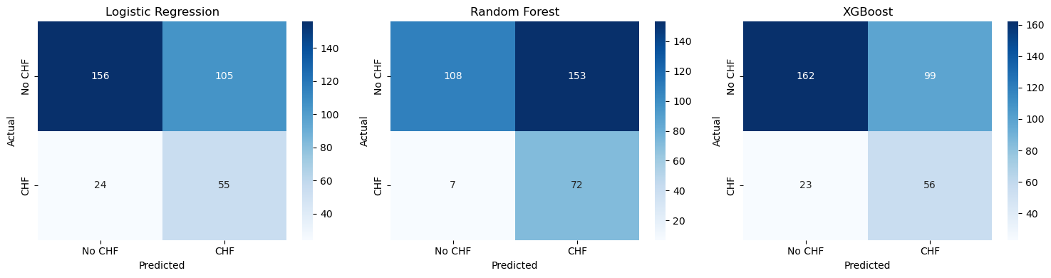
Confusion Matrix#
The confusion matrix shows the number of:
True Positives
True Negatives
False Positives
False Negatives
In clinical applications, false negatives may be particularly critical, because a high-risk patient might be missed.
fig, axes = plt.subplots(1, 3, figsize=(15,4))

for ax, (name, model) in zip(axes, models.items()):

    y_prob = model.predict_proba(X_test)[:,1]

    fpr, tpr, thresholds = roc_curve(y_test, y_prob)
    optimal_idx = np.argmax(tpr - fpr)
    optimal_threshold = thresholds[optimal_idx]

    y_pred = (y_prob >= optimal_threshold).astype(int)

    cm = confusion_matrix(y_test, y_pred)

    sns.heatmap(
        cm,
        annot=True,
        fmt="d",
        cmap="Blues",
        xticklabels=["No CHF","CHF"],
        yticklabels=["No CHF","CHF"],
        ax=ax
    )

    ax.set_title(name)
    ax.set_xlabel("Predicted")
    ax.set_ylabel("Actual")

plt.tight_layout()
plt.show()
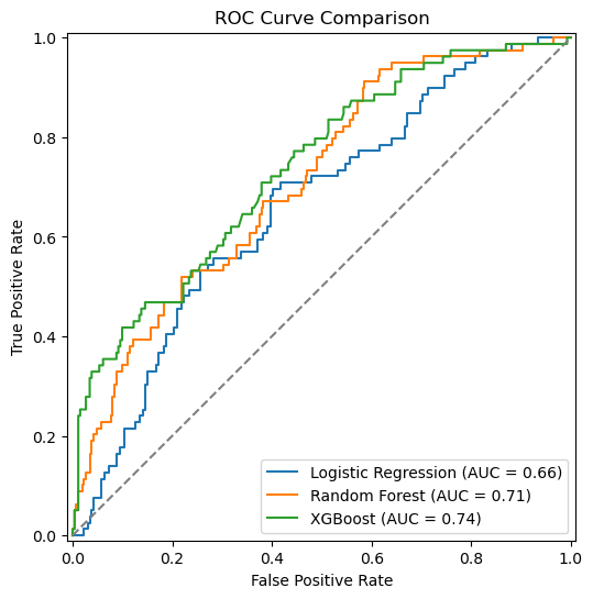
fig, ax = plt.subplots(figsize=(7,6))

for name, model in models.items():

    RocCurveDisplay.from_estimator(
        model,
        X_test,
        y_test,
        ax=ax,
        name=name
    )

# random classifier baseline
ax.plot([0,1], [0,1], linestyle="--", color="grey")

ax.set_title("ROC Curve Comparison")
ax.set_xlabel("False Positive Rate")
ax.set_ylabel("True Positive Rate")

plt.legend()
plt.show()
Optional: Model Explainability#
Machine learning models are often considered “black boxes”. To build trust in clinical AI, it is important to understand how models make predictions.
We use two approaches:
Feature Importance – which variables are most influential overall
SHAP Values – how individual features influence predictions
SHAP values allow us to interpret predictions at both the global (model-level) and local (patient-level) scale.
rf_pipeline = rf_search.best_estimator_

rf_model = rf_pipeline.named_steps["model"]

feature_names = rf_pipeline.named_steps["preprocessing"].get_feature_names_out()

importances = rf_model.feature_importances_

feature_importance = pd.DataFrame({
    "feature": feature_names,
    "importance": importances
}).sort_values("importance", ascending=False)
feature_importance.head(20)
| feature | importance | |
|---|---|---|
| 15 | cat__ZSN_A | 0.157926 |
| 0 | num__AGE | 0.092992 |
| 8 | num__ROE | 0.052270 |
| 3 | num__K_BLOOD | 0.041858 |
| 37 | cat__endocr_01 | 0.040864 |
| 6 | num__AST_BLOOD | 0.038621 |
| 17 | cat__lat_im | 0.037699 |
| 4 | num__NA_BLOOD | 0.036896 |
| 7 | num__L_BLOOD | 0.033988 |
| 40 | cat__zab_leg_01 | 0.032260 |
| 1 | num__S_AD_ORIT | 0.028063 |
| 2 | num__D_AD_ORIT | 0.023794 |
| 5 | num__ALT_BLOOD | 0.021469 |
| 20 | cat__TIME_B_S | 0.021380 |
| 47 | cat__MP_TP_POST | 0.019474 |
| 21 | cat__SEX | 0.018108 |
| 13 | cat__GB | 0.015928 |
| 16 | cat__ant_im | 0.015712 |
| 10 | cat__STENOK_AN | 0.015692 |
| 90 | cat__ANT_CA_S_n | 0.015347 |
top_features = feature_importance.head(20)

plt.figure(figsize=(8,6))

sns.barplot(
    data=top_features,
    x="importance",
    y="feature"
)

plt.title("Top 20 Feature Importances (Random Forest)")
plt.xlabel("Importance")
plt.ylabel("Feature")

plt.show()
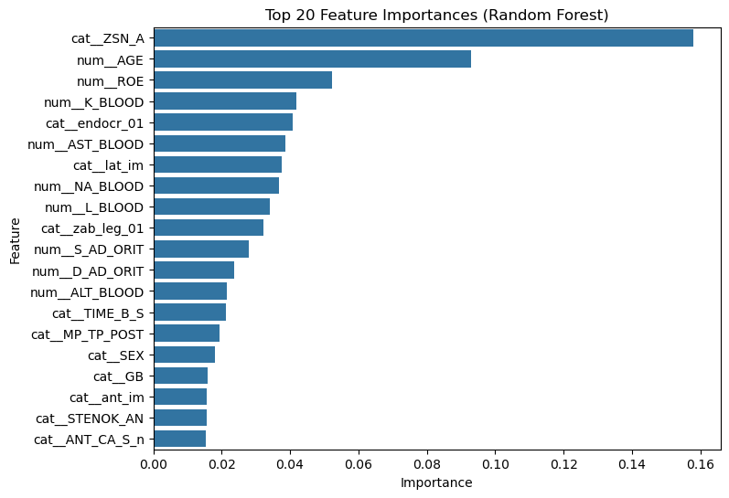
These features contribute most strongly to the model’s predictions.
Important note:
Feature importance does not necessarily indicate causality. Highly ranked variables simply help the model distinguish between patients with and without the outcome.
Discussion#
Questions to consider:
Which model performed best?
Which features were most important?
Are these findings clinically plausible?
What additional data could improve predictions?