Get the data#
We will use pandas to read a csv file which is in the same folder as your Jupyter notebook. Pandas is an open source data analysis and manipulation tool based on Python (More information: Link to website).
import pandas as pd

hb_data = pd.read_csv('HB_data.csv')
# If you want to read from a directory you can use following lines:
# from pathlib import Path
# path = Path('path-to-my-data/HB_data.csv')
# HB_data = pd.read_csv(path)

# We will look on the first 5 instances to check if it was imported successfully.
# Please note, it starts counting with 0 instead of 1:
print(f"Following data was read (showing only first 5 rows):\n{hb_data.head()}")
Following data was read (showing only first 5 rows):
    energy  bo-acc  bo-donor     q-acc   q-donor   q-hatom   dist-dh  \
0 -34.5895  0.2457    0.8981 -0.088121  0.069022  0.030216  1.029201
1 -39.2652  0.2061    0.9089 -0.100112  0.070940  0.042037  1.027247
2 -41.0025  0.1748    0.9185 -0.108372  0.072666  0.050028  1.025135
3 -40.8874  0.1496    0.9269 -0.114255  0.074115  0.055766  1.023101
4 -39.6642  0.1289    0.9341 -0.118741  0.075412  0.060208  1.021107

    dist-ah atomtype-acc atomtype-don
0  1.670799            N            N
1  1.772753            N            N
2  1.874865            N            N
3  1.976899            N            N
4  2.078893            N            N
You see 10 columns.
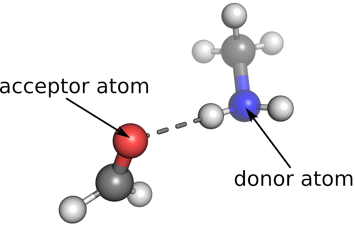
The first column is called “energy” which is the label of each instance, the hydrogen bond energy in kJ/mol.
“bo-acc” and “bo-don” are Löwdin bond orders obtained from a density functional theory calculation. A value of 1.0 means exactly one pair of electrons is shared between the respective atoms. Thus, it provides a measure of the covalent contributions to the interaction between two atoms. “bo-acc” refers to the bond order between the hydrogen atom and the hydrogen bond acceptor atom. “bo-donor” refers to the bond order between the hydrogen atom and the hydrogen bond donor atom. The latter has a higher bond order since it is a typical chemical bond and not a noncovalent interaction.
“q-acc”, “q-donor” and “q-hatom” are Löwdin partial charges in atomic units of the hydrogen bond acceptor atom, the hydrogen bond donor atom and the hydrogen bond atom, respectively.
“dist-dh” and “dist-ah” refers to the distance in Angstrom between the nucleus of the hydrogen atom and the hydrogen bond donor atom or acceptor atom.
“atomtype-acc” and “atomtype-don” refer to the element type of the hydrogen bond acceptor atom and donor atom, respectively.
You get a short description of the data type by:
hb_data.info()
<class 'pandas.core.frame.DataFrame'>
RangeIndex: 1638 entries, 0 to 1637
Data columns (total 10 columns):
 #   Column        Non-Null Count  Dtype
---  ------        --------------  -----
 0   energy        1638 non-null   float64
 1   bo-acc        1638 non-null   float64
 2   bo-donor      1638 non-null   float64
 3   q-acc         1638 non-null   float64
 4   q-donor       1638 non-null   float64
 5   q-hatom       1638 non-null   float64
 6   dist-dh       1638 non-null   float64
 7   dist-ah       1638 non-null   float64
 8   atomtype-acc  1638 non-null   object
 9   atomtype-don  1638 non-null   object
dtypes: float64(8), object(2)
memory usage: 128.1+ KB
As you can see, the atomtypes are recognized as objects while the rest are real numbers.
You can check how many instances are available for each category by:
hb_data["atomtype-acc"].value_counts()
atomtype-acc
O     990
S     288
N     216
Cl     90
F      54
Name: count, dtype: int64
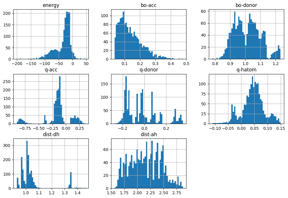
You can make a quick histogram of your numerical data by following code:
import matplotlib.pyplot as plt

hb_data.hist(bins=50, figsize=(12, 8))
plt.show()
The describe tool allows you to get a more detailed information on the numerical data:
hb_data.describe()
| energy | bo-acc | bo-donor | q-acc | q-donor | q-hatom | dist-dh | dist-ah | |
|---|---|---|---|---|---|---|---|---|
| count | 1638.000000 | 1638.000000 | 1638.000000 | 1638.000000 | 1638.000000 | 1638.000000 | 1638.000000 | 1638.000000 |
| mean | -34.783759 | 0.138418 | 1.013692 | -0.155270 | -0.022809 | 0.044391 | 1.040342 | 2.156605 |
| std | 29.955517 | 0.075418 | 0.087824 | 0.249997 | 0.151830 | 0.041812 | 0.108458 | 0.290894 |
| min | -200.597000 | 0.034200 | 0.781200 | -0.898797 | -0.275322 | -0.110008 | 0.930018 | 1.564120 |
| 25% | -48.226500 | 0.080125 | 0.942050 | -0.186461 | -0.159131 | 0.022605 | 0.978411 | 1.927490 |
| 50% | -24.801450 | 0.120600 | 1.015000 | -0.130414 | -0.036496 | 0.045868 | 1.013607 | 2.158575 |
| 75% | -14.991750 | 0.181000 | 1.073400 | -0.090575 | 0.073683 | 0.067276 | 1.038072 | 2.383549 |
| max | 45.413900 | 0.478100 | 1.232500 | 0.353389 | 0.354334 | 0.149418 | 1.459200 | 2.868591 |
std is the standard deviation of the attribute. 25%, 50% and 75% refers to the percentiles: It is the value below the given percentage of observations fall.