Train a Neural Network for Regression

This practical session will cover the building and training of a neural network. We want to work on the regression problem with the “HB energy” data to be able to compare the training process and prediction results.

The model will be built with pytorch and we do hyperparameter optimization with optuna.

Alternative libraries for hyperparameter optimization and more:

• Ray with Ray Tune

• Hyperopt

• scikit-optimize

Data preprocessing

import os
import numpy as np
import pandas as pd
import matplotlib.pyplot as plt
import math

from sklearn.model_selection import train_test_split
from sklearn.compose import ColumnTransformer
from sklearn.preprocessing import OneHotEncoder, StandardScaler, MinMaxScaler

Load and inspect data

df = pd.read_csv('data/HB_data.csv', sep=',')
display(df.head(5))
print(df.info())

	energy	bo-acc	bo-donor	q-acc	q-donor	q-hatom	dist-dh	dist-ah	atomtype-acc	atomtype-don
0	-34.5895	0.2457	0.8981	-0.088121	0.069022	0.030216	1.029201	1.670799	N	N
1	-39.2652	0.2061	0.9089	-0.100112	0.070940	0.042037	1.027247	1.772753	N	N
2	-41.0025	0.1748	0.9185	-0.108372	0.072666	0.050028	1.025135	1.874865	N	N
3	-40.8874	0.1496	0.9269	-0.114255	0.074115	0.055766	1.023101	1.976899	N	N
4	-39.6642	0.1289	0.9341	-0.118741	0.075412	0.060208	1.021107	2.078893	N	N

<class 'pandas.core.frame.DataFrame'>
RangeIndex: 1638 entries, 0 to 1637
Data columns (total 10 columns):
 #   Column        Non-Null Count  Dtype  
---  ------        --------------  -----  
 0   energy        1638 non-null   float64
 1   bo-acc        1638 non-null   float64
 2   bo-donor      1638 non-null   float64
 3   q-acc         1638 non-null   float64
 4   q-donor       1638 non-null   float64
 5   q-hatom       1638 non-null   float64
 6   dist-dh       1638 non-null   float64
 7   dist-ah       1638 non-null   float64
 8   atomtype-acc  1638 non-null   object 
 9   atomtype-don  1638 non-null   object 
dtypes: float64(8), object(2)
memory usage: 128.1+ KB
None

Check for outliers and missing data

# Have a look at the descriptive statistics
df.describe().T

	count	mean	std	min	25%	50%	75%	max
energy	1638.0	-34.783759	29.955517	-200.597000	-48.226500	-24.801450	-14.991750	45.413900
bo-acc	1638.0	0.138418	0.075418	0.034200	0.080125	0.120600	0.181000	0.478100
bo-donor	1638.0	1.013692	0.087824	0.781200	0.942050	1.015000	1.073400	1.232500
q-acc	1638.0	-0.155270	0.249997	-0.898797	-0.186461	-0.130414	-0.090575	0.353389
q-donor	1638.0	-0.022809	0.151830	-0.275322	-0.159131	-0.036496	0.073683	0.354334
q-hatom	1638.0	0.044391	0.041812	-0.110008	0.022605	0.045868	0.067276	0.149418
dist-dh	1638.0	1.040342	0.108458	0.930018	0.978411	1.013607	1.038072	1.459200
dist-ah	1638.0	2.156605	0.290894	1.564120	1.927490	2.158575	2.383549	2.868591

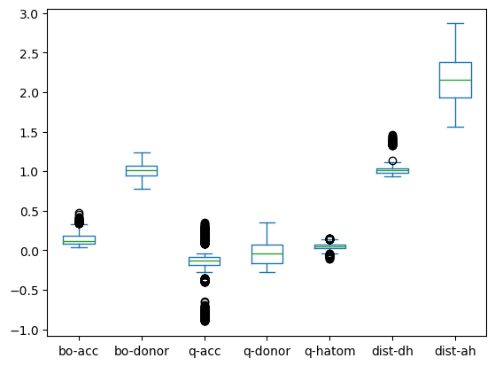
# Boxplot to have a basic check for obvious outliers
df.drop(columns=["energy"]).plot(kind="box")
plt.show()

# Check for missing values
print('Missing values:', df.isnull().sum().sum())

Missing values: 0

Prepare train and test data

We will apply similar preprocessing steps we’ve alreday seen in the regression session on day 1.
This time, we will also keep 5% of the data for a final validation on prediction quality after training.

# Get random 5% of data for validation
df_val = df.sample(frac=0.05, random_state=42)
# Drop those validation data from training data
df_tt = df.drop(df_val.index)
print(f"Training/Test data shape: {df_tt.shape}, Validation data shape: {df_val.shape}")

Training/Test data shape: (1556, 10), Validation data shape: (82, 10)

# Separate features and target
target_col = "energy"

X = df_tt.drop(columns=[target_col])
# We need y to be a 2-D array (n_samples x n_features)
y = df_tt[target_col].to_numpy().reshape(-1, 1)

# Get train and test splits
X_train, X_test, y_train, y_test = train_test_split(X, y, test_size=0.2, random_state=42)

# Preprocess and transform features
numerical_features = X.select_dtypes(include=["number"]).columns.tolist()
categorical_features = X.select_dtypes(include=["object"]).columns.tolist()

# Define scaling and encoding for X
x_preprocessor = ColumnTransformer(
    transformers=[
        ("num", StandardScaler(), numerical_features),
        ("cat", OneHotEncoder(handle_unknown="ignore", sparse_output=False), categorical_features),
    ],
    remainder="drop",
)
# Define scaling for y
y_scaler = StandardScaler()

# Fit scaling for X on train data only, apply (transform) scaling to both train and test
X_train_t = x_preprocessor.fit_transform(X_train)
X_test_t = x_preprocessor.transform(X_test)

# Fit scaling for y on train data only, apply (transform) scaling to both train and test
y_train_t = y_scaler.fit_transform(y_train)
y_test_t = y_scaler.transform(y_test)

# Get transformed feature names (handy for inspection)
feat_names = x_preprocessor.get_feature_names_out()
    
# Inspect transformed data
print("X_train: ", X_train_t.shape)
print("X_test:  ", X_test_t.shape)
print("y_train: ", y_train_t.shape)
print("y_test:  ", y_test_t.shape)
display(pd.DataFrame(X_train_t, columns=feat_names).head(5))

X_train:  (1244, 16)
X_test:   (312, 16)
y_train:  (1244, 1)
y_test:   (312, 1)

	num__bo-acc	num__bo-donor	num__q-acc	num__q-donor	num__q-hatom	num__dist-dh	num__dist-ah	cat__atomtype-acc_Cl	cat__atomtype-acc_F	cat__atomtype-acc_N	cat__atomtype-acc_O	cat__atomtype-acc_S	cat__atomtype-don_F	cat__atomtype-don_N	cat__atomtype-don_O	cat__atomtype-don_S
0	-1.285813	0.917745	-0.115091	-0.282173	0.864921	-0.662341	1.298361	0.0	0.0	0.0	1.0	0.0	0.0	0.0	1.0	0.0
1	-0.647649	0.186561	0.970476	-0.771634	-0.619231	-0.258013	1.832981	0.0	0.0	0.0	0.0	1.0	0.0	1.0	0.0	0.0
2	-1.162635	-0.394051	0.083728	-0.078369	0.426753	-0.294188	0.813984	0.0	0.0	0.0	1.0	0.0	0.0	1.0	0.0	0.0
3	0.306321	-0.886830	0.274388	0.630579	0.169388	-0.271833	-1.260058	0.0	0.0	0.0	1.0	0.0	0.0	1.0	0.0	0.0
4	2.782975	0.231048	-2.398073	-1.403848	-1.551664	-0.384992	-0.519736	1.0	0.0	0.0	0.0	0.0	0.0	0.0	1.0	0.0

pd.DataFrame(X_train_t, columns=feat_names).describe().T

	count	mean	std	min	25%	50%	75%	max
num__bo-acc	1244.0	-3.726922e-16	1.000402	-1.391955	-0.783930	-0.226356	0.561194	4.424904
num__bo-donor	1244.0	-2.077652e-16	1.000402	-2.635512	-0.825518	0.005761	0.690747	2.512432
num__q-acc	1244.0	3.212864e-17	1.000402	-2.898847	-0.137707	0.108404	0.269204	1.999119
num__q-donor	1244.0	1.427940e-18	1.000402	-1.572323	-0.879873	-0.095105	0.625609	2.481237
num__q-hatom	1244.0	-1.427940e-18	1.000402	-3.597710	-0.516487	0.048946	0.545109	2.483628
num__dist-dh	1244.0	1.115221e-15	1.000402	-1.019973	-0.572710	-0.260462	-0.034062	3.766413
num__dist-ah	1244.0	5.026347e-16	1.000402	-2.028257	-0.781578	0.003296	0.792599	2.457190
cat__atomtype-acc_Cl	1244.0	5.707395e-02	0.232077	0.000000	0.000000	0.000000	0.000000	1.000000
cat__atomtype-acc_F	1244.0	3.617363e-02	0.186797	0.000000	0.000000	0.000000	0.000000	1.000000
cat__atomtype-acc_N	1244.0	1.302251e-01	0.336686	0.000000	0.000000	0.000000	0.000000	1.000000
cat__atomtype-acc_O	1244.0	5.956592e-01	0.490961	0.000000	0.000000	1.000000	1.000000	1.000000
cat__atomtype-acc_S	1244.0	1.808682e-01	0.385064	0.000000	0.000000	0.000000	0.000000	1.000000
cat__atomtype-don_F	1244.0	5.948553e-02	0.236626	0.000000	0.000000	0.000000	0.000000	1.000000
cat__atomtype-don_N	1244.0	5.723473e-01	0.494937	0.000000	0.000000	1.000000	1.000000	1.000000
cat__atomtype-don_O	1244.0	2.636656e-01	0.440797	0.000000	0.000000	0.000000	1.000000	1.000000
cat__atomtype-don_S	1244.0	1.045016e-01	0.306033	0.000000	0.000000	0.000000	0.000000	1.000000

Build and train model with PyTorch

import torch
import torch.nn as nn
from torch.utils.data import TensorDataset, DataLoader
import torch.optim as optim
from tqdm.auto import tqdm

import optuna
optuna.logging.set_verbosity(optuna.logging.WARNING)

# Check if GPU is available to be used with pytorch
device = torch.device("cuda" if torch.cuda.is_available() else "cpu")
print(f"Using device: {device}")

Using device: cpu

Define objects for model and training process

# Define the model with a parameterizable architecture
class MLPRegressorTorch(nn.Module):
    def __init__(self, in_dim, hidden=(64, 32), dropout=0.1):
        super().__init__()
        layers = []
        prev = in_dim
        for h in hidden:
            layers += [
                # fully connected layer from prev inputs to h outputs
                nn.Linear(prev, h), 
                # non-linear activation with rectified linear unit
                nn.ReLU(), 
                # regularization via dropout: randomly zeroes activations with probability
                nn.Dropout(dropout) 
                ]
            prev = h
        # Last layer is regression output with a single neuron for continuous value
        layers += [nn.Linear(prev, 1)]
        self.net = nn.Sequential(*layers)

    def forward(self, x): 
        return self.net(x)

# Define function to create pytorch data loaders
def make_loaders(X_train_t, y_train_t, X_test_t, y_test_t, batch_size):
    # Convert data (numpy arrays) to torch tensors
    X_train_ts = torch.tensor(X_train_t, dtype=torch.float32)
    y_train_ts = torch.tensor(y_train_t, dtype=torch.float32)
    X_test_ts = torch.tensor(X_test_t, dtype=torch.float32)
    y_test_ts = torch.tensor(y_test_t, dtype=torch.float32)
    # Build torch dataset and dataloader for batches
    train_loader = DataLoader(TensorDataset(X_train_ts, y_train_ts), batch_size=batch_size, shuffle=True)
    test_loader = DataLoader(TensorDataset(X_test_ts, y_test_ts), batch_size=batch_size, shuffle=False)

    return train_loader, test_loader

# Define function for training loop with hyperparameter configuration
# Also define a directory to store model checkpoints during training
CKPT_DIR = "optuna_ckpts"
os.makedirs(CKPT_DIR, exist_ok=True)

def objective(trial):
    # Define hyperparameter search space for optuna
    hidden_layers_list = [(256, 128, 64), (128, 64), (64, 32), (64,)]
    idx = trial.suggest_int("hidden_layers_idx", 0, len(hidden_layers_list)-1)
    hidden_layers = hidden_layers_list[idx]
    dropout = trial.suggest_float("dropout", 0.0, 0.3)
    lr = trial.suggest_float("lr", 5e-4, 3e-3, log=True)
    #lr = 0.1
    weight_decay = trial.suggest_float("weight_decay", 1e-6, 1e-3, log=True)
    batch_size = trial.suggest_categorical("batch_size", [16, 32, 64, 128, 256])
    epochs = 50

    # Get data loaders for train and test data
    train_loader, test_loader = make_loaders(X_train_t, y_train_t, X_test_t, y_test_t, batch_size)

    # Initialise model and put to device (CPU or GPU)
    model = MLPRegressorTorch(
        in_dim=X_train_t.shape[1],
        hidden=hidden_layers,
        dropout=dropout
        ).to(device)
    # Define optimizer: Adam with weight decay (L2 regularization)
    optimizer = optim.Adam(model.parameters(), lr=lr, weight_decay=weight_decay)
    # Define loss function: Mean Squared Error
    loss_fn = nn.MSELoss()

    # Check model progress and store checkpoints
    best_rmse = float("inf")
    best_ckpt_path = os.path.join(CKPT_DIR, f"best_trial.pt")

    # Run epochs for training with validation at the end of each epoch
    for epoch in tqdm(range(epochs), desc="Epochs", leave=False):
        # Train for one epoch and update model parameters
        model.train()
        train_loss = 0.0
        for x_batch, y_batch in train_loader:
            x_batch, y_batch = x_batch.to(device), y_batch.to(device)
            optimizer.zero_grad()
            pred = model(x_batch)
            loss = loss_fn(pred, y_batch)
            loss.backward()
            optimizer.step()
            train_loss += loss.item() * x_batch.size(0)
        train_loss /= len(train_loader.dataset)

        # Validate in this epoch for test data without updating model parameters
        model.eval()
        val_loss = 0.0
        preds, trues = [], []
        with torch.no_grad():
            for x_batch, y_batch in test_loader:
                x_batch = x_batch.to(device)
                pred = model(x_batch)
                val_loss += loss_fn(pred, y_batch.to(device)).item() * x_batch.size(0)
                preds.append(pred.cpu().numpy())
                trues.append(y_batch.cpu().numpy())
        val_loss /= len(test_loader.dataset)

        # Get RMSE in original units (invert scaling for y)
        y_pred = y_scaler.inverse_transform(np.vstack(preds))
        y_true = y_scaler.inverse_transform(np.vstack(trues))
        val_rmse = math.sqrt(float(np.mean((y_pred - y_true) ** 2)))

        # Report to Optuna
        trial.report(val_rmse, step=epoch)
        trial.set_user_attr(f"train_loss_epoch_{epoch}", float(train_loss))
        trial.set_user_attr(f"val_loss_epoch_{epoch}", float(val_loss))
        trial.set_user_attr(f"val_rmse_epoch_{epoch}", val_rmse)
        if trial.should_prune():
            raise optuna.TrialPruned()

        # Store model checkpoint if model improved
        if val_rmse < best_rmse:
            best_rmse = val_rmse
            torch.save(
                {
                    "state_dict": model.state_dict(),
                    "model_params": {
                        "in_dim": X_train_t.shape[1],
                        "hidden": hidden_layers,
                        "dropout": dropout,
                    },
                },
                best_ckpt_path,
            )
            trial.set_user_attr("best_model_ckpt", best_ckpt_path)
            trial.set_user_attr("best_val_rmse", best_rmse)
        
    return val_rmse   

Run training with hyperparameter optimization

# Run model training and hyperparameter optimization with optuna study
study = optuna.create_study(direction="minimize")
study.optimize(objective, n_trials=20, timeout=600)

Evaluate model

best_trial = study.best_trial
best_params = best_trial.params
display("Params:", best_params)
print("Best RMSE:", best_trial.value)

'Params:'

{'hidden_layers_idx': 1,
 'dropout': 0.08436995612384487,
 'lr': 0.0027353884778077557,
 'weight_decay': 1.3565682991643851e-06,
 'batch_size': 16}

Best RMSE: 2.367166953422588

# Get all trials as DataFrame
df_all = study.trials_dataframe()

# Get best trial and its attributes
df_best = df_all[df_all["number"] == study.best_trial.number]
attrs = best_trial.user_attrs

# Collect metrics per epoch
records = []
max_epochs = max(
    int(k.split("_")[-1]) for k in attrs.keys() if "epoch" in k
) + 1

for epoch in range(max_epochs):
    record = {
        "epoch": epoch,
        "train_loss": attrs.get(f"train_loss_epoch_{epoch}"),
        "val_loss": attrs.get(f"val_loss_epoch_{epoch}"),
        "val_rmse_orig": attrs.get(f"val_rmse_epoch_{epoch}"),
    }
    if all(v is not None for v in record.values()):
        records.append(record)

df_epochs = pd.DataFrame(records).set_index("epoch")
print(df_epochs.head())

       train_loss  val_loss  val_rmse_orig
epoch                                     
0        0.212837  0.057968       7.368030
1        0.062150  0.028728       5.186882
2        0.054407  0.024758       4.815195
3        0.044266  0.022345       4.574517
4        0.037966  0.021755       4.513753

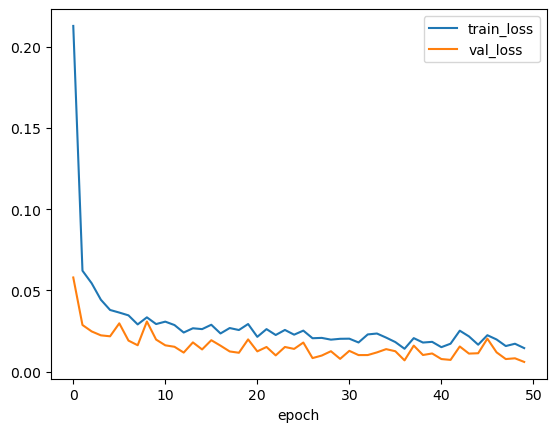
# Inspect and plot training history for best trial
display(df_epochs.info())
df_epochs[['train_loss', 'val_loss']].plot(legend=True)
plt.show()

<class 'pandas.core.frame.DataFrame'>
Index: 50 entries, 0 to 49
Data columns (total 3 columns):
 #   Column         Non-Null Count  Dtype  
---  ------         --------------  -----  
 0   train_loss     50 non-null     float64
 1   val_loss       50 non-null     float64
 2   val_rmse_orig  50 non-null     float64
dtypes: float64(3)
memory usage: 1.6 KB

None

df_epochs.val_rmse_orig.plot(legend=True)
plt.show()
print("Best RMSE: ", df_epochs.val_rmse_orig.min())

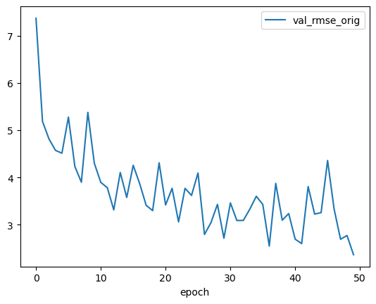
Best RMSE:  2.367166953422588

Load pretrained model and predict

Now we can load a model with our best parameter settings. We use our checkpoint for this. We finally want to predict on our validation data we sempled at the very beginning.

ckpt_path = best_trial.user_attrs["best_model_ckpt"]
ckpt = torch.load(ckpt_path, map_location=device)

# Our checkpoint contains the state dict with the trained model parameters
list(ckpt["state_dict"].items())[0]

('net.0.weight',
 tensor([[ 1.2998e-01, -5.8599e-02, -9.1701e-03,  ...,  8.2666e-02,
          -2.6167e-01, -1.7932e-01],
         [ 1.2702e-01,  6.9853e-02, -1.2293e-01,  ...,  1.6299e-02,
          -1.6481e-02, -4.8893e-04],
         [-1.5479e-02,  1.0947e-01,  6.0697e-01,  ..., -1.0442e-02,
          -1.9027e-01,  2.7875e-03],
         ...,
         [ 1.3420e-01, -5.1409e-02,  9.5353e-03,  ..., -7.1964e-02,
          -7.3765e-02, -5.6624e-02],
         [-2.4891e-01, -2.2578e-01,  4.7792e-01,  ..., -2.1212e-01,
           1.6324e-01,  2.6180e-03],
         [-1.8884e-01, -3.5862e-02, -1.8236e-01,  ..., -1.3896e-01,
          -5.1755e-02, -2.4016e-03]]))

best_model = MLPRegressorTorch(
    in_dim=ckpt["model_params"]["in_dim"],
    hidden=ckpt["model_params"]["hidden"],
    dropout=ckpt["model_params"]["dropout"],
).to(device)
best_model.load_state_dict(ckpt["state_dict"])
best_model.eval()

MLPRegressorTorch(
  (net): Sequential(
    (0): Linear(in_features=16, out_features=128, bias=True)
    (1): ReLU()
    (2): Dropout(p=0.03769065706514282, inplace=False)
    (3): Linear(in_features=128, out_features=64, bias=True)
    (4): ReLU()
    (5): Dropout(p=0.03769065706514282, inplace=False)
    (6): Linear(in_features=64, out_features=1, bias=True)
  )
)

# Separate features and target
X_val = df_val.drop(columns=["energy"])
y_val = df_val["energy"]

# Apply same scaler(s) used for training
X_val_t = x_preprocessor.transform(X_val)
y_val_t = y_scaler.transform(y_val.values.reshape(-1, 1))

# Convert to torch tensors
X_val_ts = torch.tensor(X_val_t, dtype=torch.float32).to(device)
y_val_ts = torch.tensor(y_val_t, dtype=torch.float32).to(device)

with torch.no_grad():
    y_pred_t = best_model(X_val_ts).cpu().numpy()

# Invert scaling for predictions and targets
y_pred = y_scaler.inverse_transform(y_pred_t)
y_true = y_scaler.inverse_transform(y_val_ts.cpu().numpy())

# Validate with regression metrics
from sklearn.metrics import mean_squared_error, r2_score

rmse = np.sqrt(mean_squared_error(y_true, y_pred))
r2   = r2_score(y_true, y_pred)

print(f"RMSE on validation sample: {rmse:.3f}")
print(f"R2-score on validation sample: {r2:.3f}")

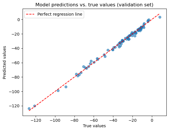
RMSE on validation sample: 2.065
R2-score on validation sample: 0.994

# Plot predictions vs true values
plt.scatter(y_true, y_pred, alpha=0.6)
plt.title("Model predictions vs. true values (validation set)")
plt.xlabel("True values")
plt.ylabel("Predicted values")
plt.plot(
    [y_true.min(), y_true.max()], 
    [y_true.min(), y_true.max()], 
    "r--", label="Perfect regression line")
plt.legend()
plt.show()