Handling missing data

When analyzing tabular data, sometimes table cells are present that do not contain data. In Python, this typically means the value is Not a Number, or NaN. We need to deal with these NaN entries differently, and this notebook will introduce how.

To get a first view where NaNs play a role, we load again some example data from a CSV file. This file uses a semicolon as separator or delimiter…we can provide pandas with this information.

import pandas as pd
import matplotlib.pyplot as plt

# Now that we know about our datatypes, we can provide this info when loading the DataFrame
# - parse timestamp to datetime and set as index
# - parse label to string, valid to boolean
df = pd.read_csv('data/converted_measuremets.csv', index_col=0, parse_dates=True, dtype={'label': 'string', 'valid': 'boolean'})
df.info()

<class 'pandas.core.frame.DataFrame'>
DatetimeIndex: 11 entries, 2023-01-01 07:00:00 to 2023-01-01 20:00:00
Data columns (total 7 columns):
 #   Column  Non-Null Count  Dtype  
---  ------  --------------  -----  
 0   label   11 non-null     string 
 1   valid   10 non-null     boolean
 2   value1  10 non-null     float64
 3   value2  8 non-null      float64
 4   value3  9 non-null      float64
 5   value4  10 non-null     float64
 6   value5  8 non-null      float64
dtypes: boolean(1), float64(5), string(1)
memory usage: 638.0 bytes

df

	label	valid	value1	value2	value3	value4	value5
timestamp
2023-01-01 07:00:00	A	True	9.0	2.0	3.1	0.98	1.23
2023-01-01 08:00:00	B	False	11.0	NaN	0.4	0.40	1.11
2023-01-01 10:00:00	D	True	9.5	5.0	NaN	2.56	NaN
2023-01-01 10:15:00	C	True	10.2	8.0	5.6	NaN	NaN
2023-01-01 11:00:00	E	False	15.0	7.0	4.4	3.14	2.34
2023-01-01 12:00:00	F	True	400.0	NaN	2.2	2.71	2.45
2023-01-01 16:00:00	G	False	9.0	1.0	1.1	3.58	0.98
2023-01-01 17:00:00	H	True	11.0	4.0	0.9	4.12	1.05
2023-01-01 18:00:00	I	True	11.3	6.0	3.3	3.33	1.67
2023-01-01 19:00:00	J	False	10.0	9.0	4.1	2.98	2.89
2023-01-01 20:00:00	K	<NA>	NaN	NaN	NaN	3.87	NaN

Examine missing data

As you can see, there are rows containing NaNs. A check if there are NaNs anywhere in a DataFrame is an important quality check at the beginning of any analysis task and good scientific practice.

Pandas’ isnull provides a boolean masking of the DataFrame with True / False values, where True indicates a NaN.

df.isnull()

	label	valid	value1	value2	value3	value4	value5
timestamp
2023-01-01 07:00:00	False	False	False	False	False	False	False
2023-01-01 08:00:00	False	False	False	True	False	False	False
2023-01-01 10:00:00	False	False	False	False	True	False	True
2023-01-01 10:15:00	False	False	False	False	False	True	True
2023-01-01 11:00:00	False	False	False	False	False	False	False
2023-01-01 12:00:00	False	False	False	True	False	False	False
2023-01-01 16:00:00	False	False	False	False	False	False	False
2023-01-01 17:00:00	False	False	False	False	False	False	False
2023-01-01 18:00:00	False	False	False	False	False	False	False
2023-01-01 19:00:00	False	False	False	False	False	False	False
2023-01-01 20:00:00	False	True	True	True	True	False	True

With this boolean masking, we can do some further analysis. And since True / False can also be interpreted as 1 / 0, we also can do math with it.

# Check if there are any NaN in the data
df.isna().values.any()

np.True_

# Get a column-wise overview of NaN and count them
df.isnull().sum().sort_values(ascending=False)

value2    3
value5    3
value3    2
valid     1
value1    1
value4    1
label     0
dtype: int64

# Compute the column-wise percentage of NaN
df.isnull().mean().sort_values(ascending=False) * 100

value2    27.272727
value5    27.272727
value3    18.181818
valid      9.090909
value1     9.090909
value4     9.090909
label      0.000000
dtype: float64

For most DataFrame methods, we can provide the parameter axis, determining whether the computation should be done on the columns or the rows / index.

# Compute the row-wise percentage of NaN
df.isnull().mean(axis=1).sort_values(ascending=False) * 100

timestamp
2023-01-01 20:00:00    71.428571
2023-01-01 10:00:00    28.571429
2023-01-01 10:15:00    28.571429
2023-01-01 08:00:00    14.285714
2023-01-01 12:00:00    14.285714
2023-01-01 07:00:00     0.000000
2023-01-01 11:00:00     0.000000
2023-01-01 16:00:00     0.000000
2023-01-01 17:00:00     0.000000
2023-01-01 18:00:00     0.000000
2023-01-01 19:00:00     0.000000
dtype: float64

We may also want to the subset of rows containing NaNs. Here, we can combine the indexing with a boolean masking for existing NaN:

df.loc[df.isnull().any(axis=1)]

	label	valid	value1	value2	value3	value4	value5
timestamp
2023-01-01 08:00:00	B	False	11.0	NaN	0.4	0.40	1.11
2023-01-01 10:00:00	D	True	9.5	5.0	NaN	2.56	NaN
2023-01-01 10:15:00	C	True	10.2	8.0	5.6	NaN	NaN
2023-01-01 12:00:00	F	True	400.0	NaN	2.2	2.71	2.45
2023-01-01 20:00:00	K	<NA>	NaN	NaN	NaN	3.87	NaN

Handling NaNs - Drop data

Depending on what kind of data analysis should be performed, it might make sense to just ignore rows and columns that contain NaN values. Alternatively, it is possible to delete rows or columns that contain NaNs. We may also use different methods to impute missing data and fill the gaps, where we should consider that those values may not represent the “real world” and may have an impact on further data analysis.

It always depends on your project, the data, and what is important or not for your analysis. It’s not an easy answer. Whatever the solution will be, it should be documented and this info should also be provided in any scientific publication based on this data.

In this case, we’ll use dropna() to remove all rows (index) which have any missing data.

df_no_nan = df.dropna(axis='index', how='any')
df_no_nan.info()

<class 'pandas.core.frame.DataFrame'>
DatetimeIndex: 6 entries, 2023-01-01 07:00:00 to 2023-01-01 19:00:00
Data columns (total 7 columns):
 #   Column  Non-Null Count  Dtype  
---  ------  --------------  -----  
 0   label   6 non-null      string 
 1   valid   6 non-null      boolean
 2   value1  6 non-null      float64
 3   value2  6 non-null      float64
 4   value3  6 non-null      float64
 5   value4  6 non-null      float64
 6   value5  6 non-null      float64
dtypes: boolean(1), float64(5), string(1)
memory usage: 348.0 bytes

We can now also check again if NaNs are present.

df_no_nan.isnull().values.any()

np.False_

Exercise

Instead of removing rows with any missing data, remove all rows that contain more than 50% of NaN. Refer to the docs for dopna() for help.

Handling NaNs - Imputation

Instead of dropping incomplete data, we can try to impute data to fill the gaps. Pandas provides basic methods to fill missing data, while other libraries also provide more sophisticated approaches, e.g.:

• scikit-learn - Imputation of missing values

# Fill missing numerical values with the mean of the column
df.fillna(df.select_dtypes(include='number').mean())

	label	valid	value1	value2	value3	value4	value5
timestamp
2023-01-01 07:00:00	A	True	9.0	2.00	3.100000	0.980	1.230
2023-01-01 08:00:00	B	False	11.0	5.25	0.400000	0.400	1.110
2023-01-01 10:00:00	D	True	9.5	5.00	2.788889	2.560	1.715
2023-01-01 10:15:00	C	True	10.2	8.00	5.600000	2.767	1.715
2023-01-01 11:00:00	E	False	15.0	7.00	4.400000	3.140	2.340
2023-01-01 12:00:00	F	True	400.0	5.25	2.200000	2.710	2.450
2023-01-01 16:00:00	G	False	9.0	1.00	1.100000	3.580	0.980
2023-01-01 17:00:00	H	True	11.0	4.00	0.900000	4.120	1.050
2023-01-01 18:00:00	I	True	11.3	6.00	3.300000	3.330	1.670
2023-01-01 19:00:00	J	False	10.0	9.00	4.100000	2.980	2.890
2023-01-01 20:00:00	K	<NA>	49.6	5.25	2.788889	3.870	1.715

# Fill missing boolean values with the most frequent one
df.fillna(df.select_dtypes(include='boolean').mode().iloc[0])

	label	valid	value1	value2	value3	value4	value5
timestamp
2023-01-01 07:00:00	A	True	9.0	2.0	3.1	0.98	1.23
2023-01-01 08:00:00	B	False	11.0	NaN	0.4	0.40	1.11
2023-01-01 10:00:00	D	True	9.5	5.0	NaN	2.56	NaN
2023-01-01 10:15:00	C	True	10.2	8.0	5.6	NaN	NaN
2023-01-01 11:00:00	E	False	15.0	7.0	4.4	3.14	2.34
2023-01-01 12:00:00	F	True	400.0	NaN	2.2	2.71	2.45
2023-01-01 16:00:00	G	False	9.0	1.0	1.1	3.58	0.98
2023-01-01 17:00:00	H	True	11.0	4.0	0.9	4.12	1.05
2023-01-01 18:00:00	I	True	11.3	6.0	3.3	3.33	1.67
2023-01-01 19:00:00	J	False	10.0	9.0	4.1	2.98	2.89
2023-01-01 20:00:00	K	True	NaN	NaN	NaN	3.87	NaN

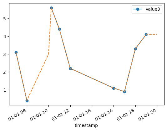
# We can also try to interpolate missing values
df['value3'].plot(style="o-", legend=True)
# Interpolate privides different methods, e.g linear, quadratic, etc
df['value3'].interpolate(method='linear').plot(style="--")
plt.show()

Exercise

Lets combine all this to

• fill missing boolean values via mode

• fill missing numerical values by linear interpolation

You may want to consider the use of apply(), to apply according methods to each column.

Save the result to data/filled_measurements.csv