Present and store your model#
We have identified and optimized our best model by cross-validation. We train this model on the full training data now.
# code from previous notebooks of this section
import pandas as pd
from sklearn.model_selection import train_test_split
from sklearn.ensemble import GradientBoostingRegressor
from sklearn.svm import SVR
from sklearn.pipeline import make_pipeline
from sklearn.preprocessing import StandardScaler
from sklearn.preprocessing import OneHotEncoder
from sklearn.compose import ColumnTransformer
from sklearn.compose import make_column_selector
import numpy as np

hb_data = pd.read_csv('HB_data.csv')
train_set, test_set = train_test_split(hb_data, test_size=0.2, random_state=42)

y_train = train_set['energy']
X_train = train_set.drop(['energy'], axis=1)

num_pipeline = make_pipeline(StandardScaler())
cat_pipeline = make_pipeline(OneHotEncoder(sparse_output=False))

preprocessing = ColumnTransformer([("num",num_pipeline, make_column_selector(dtype_include=np.number)),
                                        ("cat",cat_pipeline, make_column_selector(dtype_include=object)),])
# end code from previous notebooks of this section

model_final = make_pipeline(preprocessing,GradientBoostingRegressor(init=SVR(kernel="rbf", C=5000, epsilon=0.1), random_state=42,
                                  learning_rate=0.1, n_estimators=70, max_depth=5, min_samples_split=2))

model_final.fit(X_train,y_train)
Pipeline(steps=[('columntransformer',
                 ColumnTransformer(transformers=[('num',
                                                  Pipeline(steps=[('standardscaler',
                                                                   StandardScaler())]),
                                                  <sklearn.compose._column_transformer.make_column_selector object at 0x79b2fe78ac00>),
                                                 ('cat',
                                                  Pipeline(steps=[('onehotencoder',
                                                                   OneHotEncoder(sparse_output=False))]),
                                                  <sklearn.compose._column_transformer.make_column_selector object at 0x79b2fdee4b30>)])),
                ('gradientboostingregressor',
                 GradientBoostingRegressor(init=SVR(C=5000), max_depth=5,
                                           n_estimators=70, random_state=42))])
In a Jupyter environment, please rerun this cell to show the HTML representation or trust the notebook. On GitHub, the HTML representation is unable to render, please try loading this page with nbviewer.org.
Parameters
| steps | [('columntransformer', ...), ('gradientboostingregressor', ...)] | |
| transform_input | None | |
| memory | None | |
| verbose | False |
Parameters
| transformers | [('num', ...), ('cat', ...)] | |
| remainder | 'drop' | |
| sparse_threshold | 0.3 | |
| n_jobs | None | |
| transformer_weights | None | |
| verbose | False | |
| verbose_feature_names_out | True | |
| force_int_remainder_cols | 'deprecated' |
<sklearn.compose._column_transformer.make_column_selector object at 0x79b2fe78ac00>
Parameters
| copy | True | |
| with_mean | True | |
| with_std | True |
<sklearn.compose._column_transformer.make_column_selector object at 0x79b2fdee4b30>
Parameters
| categories | 'auto' | |
| drop | None | |
| sparse_output | False | |
| dtype | <class 'numpy.float64'> | |
| handle_unknown | 'error' | |
| min_frequency | None | |
| max_categories | None | |
| feature_name_combiner | 'concat' |
Parameters
| loss | 'squared_error' | |
| learning_rate | 0.1 | |
| n_estimators | 70 | |
| subsample | 1.0 | |
| criterion | 'friedman_mse' | |
| min_samples_split | 2 | |
| min_samples_leaf | 1 | |
| min_weight_fraction_leaf | 0.0 | |
| max_depth | 5 | |
| min_impurity_decrease | 0.0 | |
| init | SVR(C=5000) | |
| random_state | 42 | |
| max_features | None | |
| alpha | 0.9 | |
| verbose | 0 | |
| max_leaf_nodes | None | |
| warm_start | False | |
| validation_fraction | 0.1 | |
| n_iter_no_change | None | |
| tol | 0.0001 | |
| ccp_alpha | 0.0 |
SVR(C=5000)
Parameters
| kernel | 'rbf' | |
| degree | 3 | |
| gamma | 'scale' | |
| coef0 | 0.0 | |
| tol | 0.001 | |
| C | 5000 | |
| epsilon | 0.1 | |
| shrinking | True | |
| cache_size | 200 | |
| verbose | False | |
| max_iter | -1 |
And we can validate our model on the test data set which was never used during the model development.
from sklearn.metrics import mean_absolute_error
from sklearn.metrics import max_error
from sklearn.metrics import mean_absolute_percentage_error
from sklearn.metrics import root_mean_squared_error
from sklearn.metrics import r2_score

y_test = test_set['energy']
X_test = test_set.drop(['energy'], axis=1)

final_predictions = model_final.predict(X_test)
final_mae = mean_absolute_error(y_test, final_predictions)
print("The model has a mean absolute error of %0.2f kJ/mol on the test data set\n" % final_mae)
final_maep = mean_absolute_percentage_error(y_test, final_predictions)
print("The model has a mean absolute percentage error of %0.2f on the test data set\n" % final_maep)
final_rmse = root_mean_squared_error(y_test, final_predictions)
print("The model has a root mean square error of %0.2f kJ/mol on the test data set\n" % final_rmse)
final_max = max_error(y_test, final_predictions)
print("The model has a maximum residual error of %0.2f kJ/mol on the test data set\n" % final_max)
final_r2 = r2_score(y_test, final_predictions)
print("The model has a coefficient of determination of %0.3f on the test data set\n" % final_r2)
The model has a mean absolute error of 0.51 kJ/mol on the test data set

The model has a mean absolute percentage error of 0.03 on the test data set

The model has a root mean square error of 0.85 kJ/mol on the test data set

The model has a maximum residual error of 4.23 kJ/mol on the test data set

The model has a coefficient of determination of 0.999 on the test data set
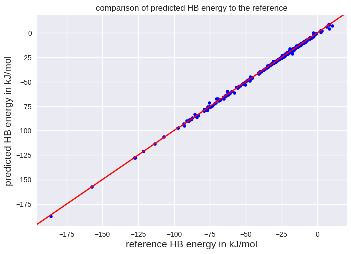
We see that the root mean squared error is 0.85 kJ/mol. The smaller value compared to the cross-validation seems reasonable since we used a larger data set to train the model. We can also visualize the performance of our model by a scatter plot:
import matplotlib.pyplot as plt

plt.style.use('seaborn-v0_8')

# The next line will add y=x to our graph
plt.axline((0, 0), slope=1, color='r')
plt.scatter(y_test, final_predictions, color='b', s=20)
plt.xlabel("reference HB energy in kJ/mol", fontsize=14)
plt.ylabel("predicted HB energy in kJ/mol", fontsize=14)
plt.title("comparison of predicted HB energy to the reference")

plt.show()
We can store our model by:
import joblib

joblib.dump(model_final, "HB_energy.pkl")
['HB_energy.pkl']
You can use it later by:
import joblib

y_test = test_set['energy']
X_test = test_set.drop(['energy'], axis=1)

final_model_reloaded = joblib.load("HB_energy.pkl")

test_stored_model = final_model_reloaded.predict(X_test)
final_mae = mean_absolute_error(y_test, test_stored_model)
print("The model has a mean absolute error of %0.2f kJ/mol on the test data set\n" % final_mae)
The model has a mean absolute error of 0.51 kJ/mol on the test data set