Delayed processing with Dask#
In this notebook we will work with a dataset that exceeds the amount of available memory. The trick is to use Dask delayed processing capabilities.
import numpy as np
import dask
import dask.array as da
from dask import delayed
import matplotlib.pyplot as plt
import stackview
from timeit import timeit

# see mandelbrot.py
from mandelbrot import mandelbrot_array
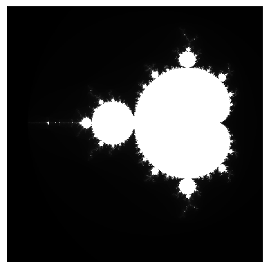
As example, we use the mandelbrot set that can be visualized as images with various zoom levels.
stackview.imshow(mandelbrot_array(scale=3))
stackview.insight(mandelbrot_array(scale=0.01))

|

|
Compute time considerations#
First, we use timeit to measure how long the computation of one image takes.
%%timeit
mandelbrot_array()
215 ms ± 7.73 ms per loop (mean ± std. dev. of 7 runs, 1 loop each)
If computing a single image takes 0.3 seconds, and we need to compute 200000 images, this will take a while.
single_image_time = 0.3
number_of_images = 200000

single_image_time * number_of_images / 60 / 60, "h"
(16.666666666666668, 'h')
Hence, if we wanted to generate a stack of images where we can zoom in, this might take hours.
Delayed processing#
A way to deal with long compute times is delayed processing. Goal of this technique is to have a dataset ready for manual inspection, e.g. viewing individual slice of the data, and handle it as a normmal array or Dask stack.
The first step is to delay a function, by decorating it with @delayed.
@delayed
def render_level(i):
    from mandelbrot import SCALE0, ZOOM_PER_LEVEL
    scale = SCALE0 / (ZOOM_PER_LEVEL ** i)
    return mandelbrot_array(scale=scale)
Next, we create a list of delayed objects and turn this list into a stack. A stack is n+1 dimensional arrays with dimensionality n.
from mandelbrot import WIDTH, HEIGHT, SCALE0
DTYPE = np.uint16
CHUNKS = (1, 256, 256)

levels = [
    da.from_delayed(
        render_level(i),
        shape=(HEIGHT, WIDTH), dtype=DTYPE
    )
    for i in range(number_of_images)
]
stack = da.stack(levels, axis=0)
In Jupyter notebooks, such a stack renders a preview specifying how the data looks like. Note that until here, no Mandelbrot images was computed yet.
stack
|
||||||||||||||||
We can also show individual slices in the stack.
stackview.imshow(stack[0])
type(stack[0])
dask.array.core.Array
We can also generate animations from the images in this huge stack. In the following, we compute 20 slices, which take some time.
image = np.asarray(stack[0:20000:1000,::2,::2])
image.shape
(20, 256, 256)
stackview.animate(image)
C:\Users\rober\miniforge3\envs\bob-env\Lib\site-packages\stackview\_animate.py:43: UserWarning: The timelapse has an intensity range exceeding 0..255. Consider normalizing it to the range between 0 and 255.
  warnings.warn("The timelapse has an intensity range exceeding 0..255. Consider normalizing it to the range between 0 and 255.")

Exercise#
Find the first image in the stack where all pixels values have the same intensity.
stack.shape
(200000, 512, 512)
stackview.imshow(stack[0])
stackview.imshow(stack[-1])