Image visualization with stackview

In this notebook we will learn how to visualize images using stackview.

Most of the tools used here will not render in the website. You must execute this notebook locally to make use of stackview.

Usage

You can use stackview from within jupyter notebooks as shown below.

import stackview

from skimage.io import imread, imshow

First we load an example image. The ´imread´ function allows to open common file formats such as TIF. To get a first glimps about the data, we print out its dimensionality using ´.shape´.

image = imread("../day2.1_image_segmentation/data/BMP4blastocystC3-cropped_resampled_8bit.tif")
image.shape

(86, 396, 393)

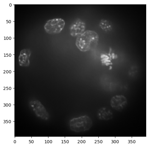
A common way for visualizing images is using the imshow function. It only works for 2D images and thus, we need to select a slice, for example the center slice.

center_slice = int(image.shape[0] / 2)

imshow(image[center_slice])

<matplotlib.image.AxesImage at 0x1ae8b7f02b0>

To get better overview about the image, its size and pixel intensity distribution, we use the stackview.insight function. Note that this is a 3D image. We are looking at a maximum intensity projection along the z-axis.

stackview.insight(image)

shape (86, 396, 393) dtype uint8 size 12.8 MB min 0 max 255

Slice

You can also view it slice-by-slice. Note: This view will not render on the course website. You need to run the code locally or on the Jupyter-Hub of your institute, e.g. at Uni-Leipzig.

stackview.slice(image)

Picker

To read the intensity of pixels where the mouse is moving, use the picker.

stackview.picker(image)

Curtain

For visualization of an original image in combination with segmented image, the ´curtain´ may be helpful. Note: This segmentation just serves as example. We can do much better than that.

binary_image = image > 80

stackview.curtain(image, binary_image)

The curtain can also be partially transparent using the alpha value.

stackview.curtain(image, binary_image, alpha=0.3)

The curtain also works with 2D data

Switch

If there are many images you would like to inspect, for example fluorescent channels, you can pass them as dictionary or list to switch().

hela_cells = imread("../data/hela-cells.tif")
hela_cells.shape

(512, 672, 3)

From ´.shape´ we can read the dimensions of the image. Obvisouly, this image has three channels. We can extract these channels using what we learned about arrays: indexing.

# take the time and give variables good names.
# For example, when extracting channels, give them biologically meaningful names
lysosomes_channel = hela_cells[:,:,0]
mitochondria_channel = hela_cells[:,:,1]
nuclei_channel = hela_cells[:,:,2]

# and check that the name make sense.
stackview.insight(nuclei_channel)

shape (512, 672) dtype uint16 size 672.0 kB min 0 max 2832

Then, we can pass the channel images and corresponding descriptive names.

stackview.switch(
    {
        "Lysosomes":   lysosomes_channel,
        "Mitochondria":mitochondria_channel,
        "Nuclei":      nuclei_channel
    }
)

You can also configure corresponding color maps and show multiple channels at a time. You find an overview about possible colormaps here. Additionally, color maps called pure_ and a color are available.

stackview.switch(
    {
        "Lysosomes":   lysosomes_channel,
        "Mitochondria":mitochondria_channel,
        "Nuclei":      nuclei_channel
    },
    colormap=[
        "pure_magenta", 
        "pure_green", 
        "pure_blue"
    ],
    toggleable=True
)

Exercise 1

Modify the code above to visualize the Hela nuclei in red and the mitochondria in cyan.

Exercise 2

Use the picker tool to get an idea about the intensity in the nuclei.

Optional Exercise:

Open an own multi-channel file and visualize its content.