Image Processing Filters

Filters are mathematical operations that produce a new image out of one or more images. Pixel values between input and output images may differ.

import numpy as np

import matplotlib.pyplot as plt
from skimage.io import imread
from skimage import data
from skimage import filters
from skimage import morphology
from scipy.ndimage import convolve, gaussian_laplace
import stackview

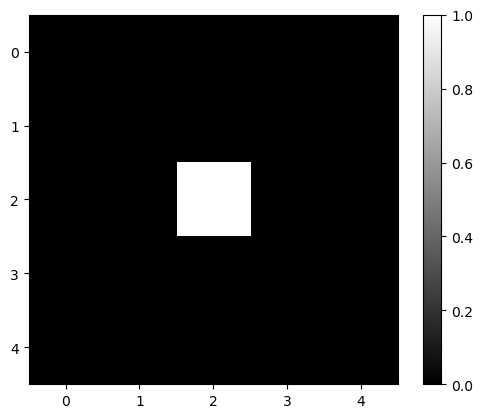
To demonstrate what specific filters do, we start with a very simple image. It contains a lot of zeros and a single pixel with value 1 in the middle.

image1 = np.zeros((5, 5))
image1[2, 2] = 1
image1

array([[0., 0., 0., 0., 0.],
       [0., 0., 0., 0., 0.],
       [0., 0., 1., 0., 0.],
       [0., 0., 0., 0., 0.],
       [0., 0., 0., 0., 0.]])

plt.imshow(image1, cmap='gray')
plt.colorbar()

<matplotlib.colorbar.Colorbar at 0x7f1301b62a30>

Gaussian kernel

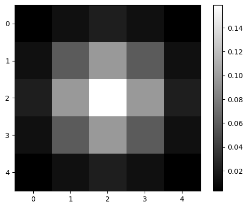
To apply a Gaussian blur to an image, we convolve it using a Gaussian kernel. The function gaussian in scikit-image can do this for us.

blurred = filters.gaussian(image1, sigma=1)
blurred

array([[0.00291504, 0.01306431, 0.02153941, 0.01306431, 0.00291504],
       [0.01306431, 0.05855018, 0.09653293, 0.05855018, 0.01306431],
       [0.02153941, 0.09653293, 0.15915589, 0.09653293, 0.02153941],
       [0.01306431, 0.05855018, 0.09653293, 0.05855018, 0.01306431],
       [0.00291504, 0.01306431, 0.02153941, 0.01306431, 0.00291504]])

plt.imshow(blurred, cmap='gray')
plt.colorbar()

<matplotlib.colorbar.Colorbar at 0x7f1301a91790>

Laplacian

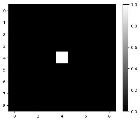
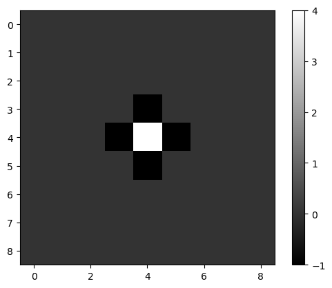
Whenever you wonder what a filter might be doing, just create a simple test image and apply the filter to it.

image2 = np.zeros((9, 9))
image2[4, 4] = 1

plt.imshow(image2, cmap='gray')
plt.colorbar()

<matplotlib.colorbar.Colorbar at 0x7f13019d6460>

mexican_hat = filters.laplace(image2)

plt.imshow(mexican_hat, cmap='gray')
plt.colorbar()

<matplotlib.colorbar.Colorbar at 0x7f130178df10>

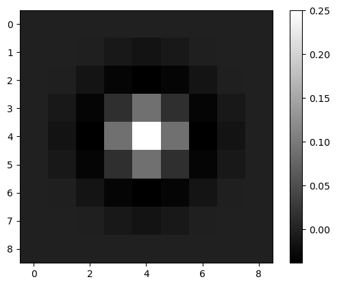
Laplacian of Gaussian

We can also combine filters, e.g. using functions. If we apply a Gaussian filter to an image and a Laplacian afterwards, we have a filter doing the Laplacian of Gaussian (LoG) per definition.

def laplacian_of_gaussian(image, sigma):
    """
    Applies a Gaussian kernel to an image and the Laplacian afterwards.
    """
    
    # blur the image using a Gaussian kernel
    intermediate_result = filters.gaussian(image, sigma)
    
    # apply the mexican hat filter (Laplacian)
    result = filters.laplace(intermediate_result)
    
    return result

log_image1 = laplacian_of_gaussian(image2, sigma=1)

plt.imshow(log_image1, cmap='gray')
plt.colorbar()

<matplotlib.colorbar.Colorbar at 0x7f13016dcd30>

Interactive filter parameter tuning

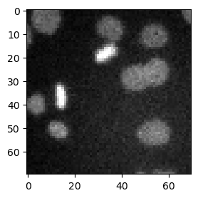
To understand better what filters are doing, it shall be recommended to apply them interactively. The following code will not render on github.com. You need to execute the notebook locally use this interactive user-interface.

image3 = imread('data/mitosis_mod.tif').astype(float)

plt.figure(figsize=(3,3))
plt.imshow(image3, cmap = 'gray')

<matplotlib.image.AxesImage at 0x7f1301608610>

stackview.interact(laplacian_of_gaussian, image3, zoom_factor=4)

More filter examples

We demonstrate some more typical filters using this nuclei example image.

Denoising

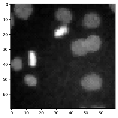
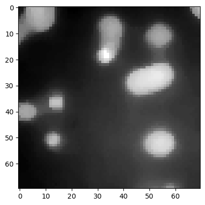
Common filters for denoising images are the mean filter, the median filter and the Gaussian filter. For the non linear filters mean and median, we have to define the neighborhood for calculation.

denoised_mean = filters.rank.mean(image3.astype(np.uint8), morphology.disk(1))

plt.imshow(denoised_mean, cmap='gray')

<matplotlib.image.AxesImage at 0x7f130113dcd0>

morphology.disk(1)

array([[0, 1, 0],
       [1, 1, 1],
       [0, 1, 0]], dtype=uint8)

denoised_median = filters.median(image3, morphology.disk(1))

plt.imshow(denoised_median, cmap='gray')

<matplotlib.image.AxesImage at 0x7f1300f5d9a0>

denoised_median2 = filters.median(image3, morphology.disk(5))

plt.imshow(denoised_median2, cmap='gray')

<matplotlib.image.AxesImage at 0x7f1300edcf10>

denoised_gaussian = filters.gaussian(image3, sigma=1)

plt.imshow(denoised_gaussian, cmap='gray')

<matplotlib.image.AxesImage at 0x7f1300e5c970>

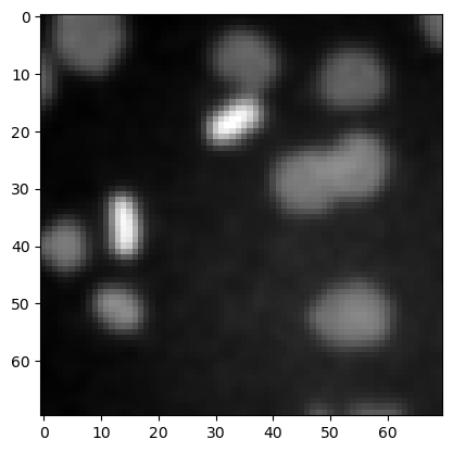
We can also show these images side-by-side using matplotlib.

fig, axes = plt.subplots(1,3, figsize=(15,15))

axes[0].imshow(denoised_mean, cmap='gray')
axes[1].imshow(denoised_median, cmap='gray')
axes[2].imshow(denoised_gaussian, cmap='gray')

<matplotlib.image.AxesImage at 0x7f1300ddef40>

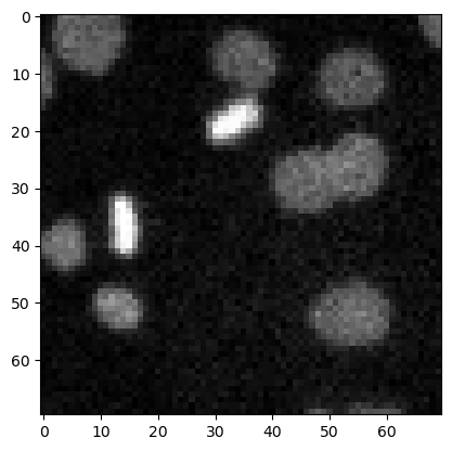
Top-hat filtering / background removal

top_hat = morphology.white_tophat(image3, morphology.disk(15))

plt.imshow(top_hat, cmap='gray')

<matplotlib.image.AxesImage at 0x7f1300434820>

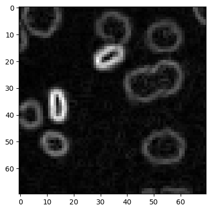
Edge detection

sobel = filters.sobel(image3)

plt.imshow(sobel, cmap='gray')

<matplotlib.image.AxesImage at 0x7f1300d022e0>

Custom kernel

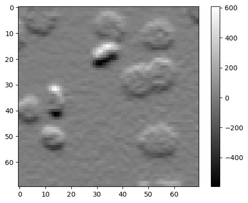
When applying linear filters such as Gaussian and Laplacian, we technically convole the image. We can also convolve it using a custom kernel.

kernel1 = [[1, 2, 1],
           [0, 0, 0],
           [-1, -2, -1]]

output1 = convolve(image3, kernel1)

plt.imshow(output1, cmap='gray')
plt.colorbar()

<matplotlib.colorbar.Colorbar at 0x7f1301927be0>

Exercise 1

The above filter hightlights horizontal edges in the image. Write code that highlights vertical edges.

Hint: read more about the Sobel operator.

Exercise 2

Write a function that computes the Difference of Gaussian.

def difference_of_gaussian(image, sigma1, sigma2):
    # enter code here

Use a simple function call to try out the function.

dog_image = difference_of_gaussian(image3, 1, 5)

plt.imshow(dog_image, cmap='gray')

Use the stackview library to play with it interactively.

stackview.interact(difference_of_gaussian, image3, zoom_factor = 4)