Part 3: Machine Learning insights by Data Viz

import warnings
warnings.simplefilter(action='ignore', category=FutureWarning) ## suppress annoying deprecation warnings

import pandas as pd
import seaborn.objects as so
import seaborn as sns
import matplotlib.pyplot as plt


from sklearn import tree
from sklearn.ensemble import RandomForestClassifier
from sklearn.metrics import confusion_matrix, ConfusionMatrixDisplay
from sklearn.model_selection import cross_validate

# Renaming columns for better axis labels in plots

col_rename = {
	'tavg': 'Temp_Avg_°C',
	'tmax': 'Temp_Max_°C',
	'tmin': 'Temp_Min_°C',
	'rhum': 'Rel_Humidity_%',
	'coco': 'Condition',
	'wspd': 'Wind_Speed_kmh',
	'prcp': 'Precipation_mm',
	'wdir': 'Wind_Direction_°',
	'pres': 'Air_pressure_hPa',
	'dwpt': 'Dew_point_°C'
}

## Reload data
weather_df = pd.read_csv('global_weather.csv', parse_dates=['time'], dtype={'wmo':str, 'station':str}) 
weather_df = weather_df.dropna()

weather_df.rename(columns=col_rename, inplace=True)
weather_df = weather_df.assign(Continent = weather_df["timezone"].str.split('/').str[0])  ## Get continent from timezone column

Plotting feature correlation: first try

weather_corr = weather_df.select_dtypes(include='number').corr() ## Calculate (Pearson) correlation for all numerical features in dataframe

f, ax = plt.subplots(figsize=(11, 9))
#!# sns.??(weather_corr, ## seaborn.object no function for heatmaps yet
sns.heatmap(weather_corr, ## seaborn.object no function for heatmaps yet
			cbar_kws={"label": "Pearson correlation coefficient", "shrink": 0.6} ## Label adjustments
			) 

<Axes: >

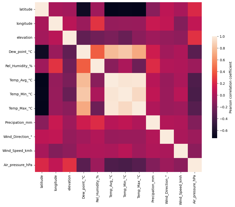
Problem with standard correlation heatmap: colormap not suitable and features not ordered by similarity

sns.clustermap(weather_corr,                                            ## Clustermap will cluster the features by similarity
			    cmap='vlag',center=0, vmin=-1, vmax=1,                  ## Colormap: correlations range from -1 to +1 and have fixed midpoint at 0                                  
				cbar_kws={"label": "Pearson correlation coefficient"},  ## Color legend description
                cbar_pos = (0.05, 0.45, 0.03, 0.2)						## Change the weird default position of legend
				).ax_row_dendrogram.set_visible(False)					## Dendrogram of feature similarity is identical (symmetric matrix); we can omit it on one side

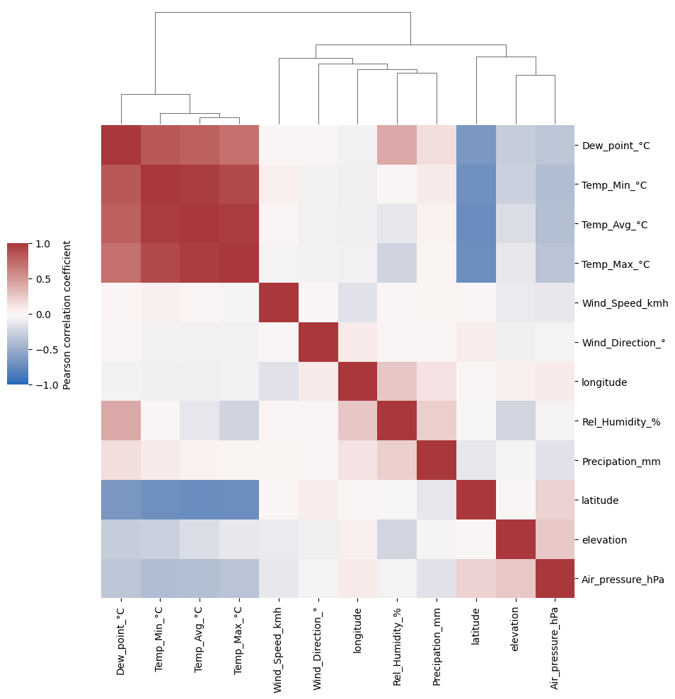
What can be seen in the correlation heatmap?

(1) features with (almost) identical information (redundancy)
(2) association of learned embeddings (t-SNE, PCA) with features

ML show case: predict the manuel text annotation of the weather by the numerical features

weather_df['Condition'].value_counts()

Condition
Cloudy               827
Fair                 734
Clear                557
Overcast             239
Light Rain           108
Fog                  105
Rain                  69
Heavy Rain Shower     60
Heavy Rain            50
Rain Shower           29
Thunderstorm          19
Light Snowfall        11
Snow Shower            4
Sleet                  3
Snowfall               3
Heavy Snowfall         3
Heavy Snow Shower      3
Heavy Sleet            1
Name: count, dtype: int64

For simplicity reducing to Top categories

weather_df_red = weather_df[
	weather_df['Condition'].isin( 
		weather_df['Condition'].value_counts()[0:6].index  ## Top categories
		) 
	]

weather_df_red

	name	country	region	wmo	icao	latitude	longitude	elevation	timezone	hourly_start	...	Rel_Humidity_%	Condition	Temp_Avg_°C	Temp_Min_°C	Temp_Max_°C	Precipation_mm	Wind_Direction_°	Wind_Speed_kmh	Air_pressure_hPa	Continent
1	Peshawar	PK	N	41530	OPPS	34.0167	71.5833	359.0	Asia/Karachi	1944-01-01	...	100.0	Clear	10.8	9.0	12.5	65.0	12.0	11.7	1005.5	Asia
2	Peshawar	PK	N	41530	OPPS	34.0167	71.5833	359.0	Asia/Karachi	1944-01-01	...	94.0	Cloudy	8.9	5.5	13.0	16.0	330.0	20.4	1012.6	Asia
3	Peshawar	PK	N	41530	OPPS	34.0167	71.5833	359.0	Asia/Karachi	1944-01-01	...	54.0	Fair	11.3	4.5	18.0	0.0	270.0	14.2	1020.1	Asia
4	Peshawar	PK	N	41530	OPPS	34.0167	71.5833	359.0	Asia/Karachi	1944-01-01	...	50.0	Fog	13.7	5.5	21.5	0.0	222.0	13.7	1019.3	Asia
5	Peshawar	PK	N	41530	OPPS	34.0167	71.5833	359.0	Asia/Karachi	1944-01-01	...	51.0	Fog	14.9	6.0	21.5	0.0	222.0	8.1	1015.7	Asia
...	...	...	...	...	...	...	...	...	...	...	...	...	...	...	...	...	...	...	...	...	...
3687	Fuerteventura / Aeropuerto	ES	CN	60035	GCFV	28.4500	-13.8667	22.0	Europe/Madrid	1950-03-27	...	78.0	Clear	19.9	16.7	22.0	0.0	32.0	12.2	1018.1	Europe
3688	Fuerteventura / Aeropuerto	ES	CN	60035	GCFV	28.4500	-13.8667	22.0	Europe/Madrid	1950-03-27	...	57.0	Fair	23.0	18.8	28.0	0.0	0.0	12.5	1016.2	Europe
3689	Fuerteventura / Aeropuerto	ES	CN	60035	GCFV	28.4500	-13.8667	22.0	Europe/Madrid	1950-03-27	...	73.0	Clear	21.9	20.0	26.0	0.0	331.0	27.7	1016.2	Europe
3690	Fuerteventura / Aeropuerto	ES	CN	60035	GCFV	28.4500	-13.8667	22.0	Europe/Madrid	1950-03-27	...	69.0	Fair	20.2	18.0	23.0	0.0	19.0	24.9	1017.0	Europe
3691	Fuerteventura / Aeropuerto	ES	CN	60035	GCFV	28.4500	-13.8667	22.0	Europe/Madrid	1950-03-27	...	47.0	Fair	20.2	17.4	24.0	0.0	6.0	29.7	1018.5	Europe

2570 rows × 28 columns

X = weather_df_red.select_dtypes(include='number') 	## Define features
#!# y = weather_df_red[??]  				## Define target variable
y = weather_df_red['Condition']  				## Define target variable

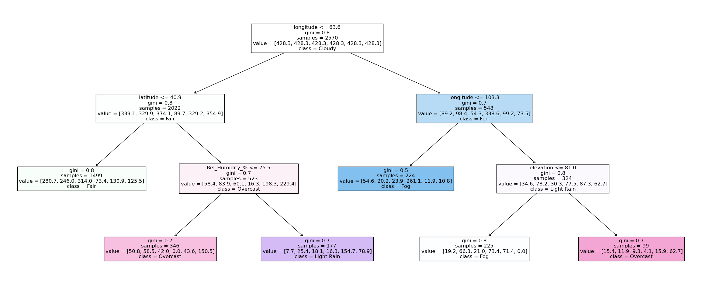
clf = tree.DecisionTreeClassifier(max_depth=5,class_weight="balanced", max_leaf_nodes = 6) ## Define a simple decision tree

clf = clf.fit(X, y)		## training

plt.figure(figsize=(30,12))  ## Plot the full decision tree
anno = tree.plot_tree(	clf, 									## Decision tree
			   	feature_names=clf.feature_names_in_.tolist(),	## Features names
			   	class_names = clf.classes_.tolist(),			## Weather condition text
				filled = True,									## Colored by class decision
				impurity =True,								## For simiplicity exclude impurity values at splits
				precision=1,									## decimal precision
				fontsize=12)									## Fontsize for readibility

Insights into more complex ML models: Random Forest

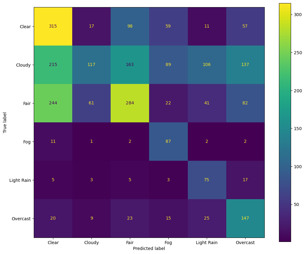
Plotting results: confusion matrix

Important for Confusion Matrix visualization is color + number per entry for pattern exploration and precision

clf_rf = RandomForestClassifier(n_estimators=100,  class_weight="balanced", max_leaf_nodes=20) ## What happens if we negelect class imbalance?
#!# clf_rf = RandomForestClassifier(n_estimators=100,  class_weight=None, max_leaf_nodes=20) ## What happens if we negelect class imbalance?


output = cross_validate(clf_rf, X, y, cv=5, scoring = 'accuracy', return_estimator =True) ## RandomForest is non-deterministic ML -> Cross-validation for more robust results

clf_rf_1 = output['estimator'][0] ## Select a learned RF from the cross-validation

y_pred = clf_rf_1.predict(X)
labels = clf_rf_1.classes_.tolist()
cm = confusion_matrix(y, y_pred, labels=labels)
fig, ax = plt.subplots(figsize=(12,10))
ConfusionMatrixDisplay(confusion_matrix=cm, display_labels=labels).plot(ax=ax) 

<sklearn.metrics._plot.confusion_matrix.ConfusionMatrixDisplay at 0x7fa249222430>

Getting explainability from feature importance

Extracting importance from learned models across all cross validations for robustness

feature_importances = pd.DataFrame(X.columns.to_list(), index = X.columns.to_list(), columns=['feature']) ## Empty Data frame definition

for idx,estimator in enumerate(output['estimator']):  ## For each tree in RF
    feature_importances = feature_importances.join(         
            pd.DataFrame(estimator.feature_importances_ ,             ## Calculated feature importance
                        index = estimator.feature_names_in_.tolist(), ## Feature Names
                        columns=['importance_cv'+str(idx+1)])         ## Save from which CV split
            )

# feature_importances
#!# feature_importances_long = pd.??( feature_importances, stubnames="importance_cv",i="feature",j="cv") 
feature_importances_long = pd.wide_to_long( feature_importances, stubnames="importance_cv",i="feature",j="cv") 

feature_importances_long.head() ## We need typically long format for plotting in grammar of graphics

		importance_cv
feature	cv
latitude	1	0.124856
longitude	1	0.203709
elevation	1	0.066899
Dew_point_°C	1	0.051925
Rel_Humidity_%	1	0.136801

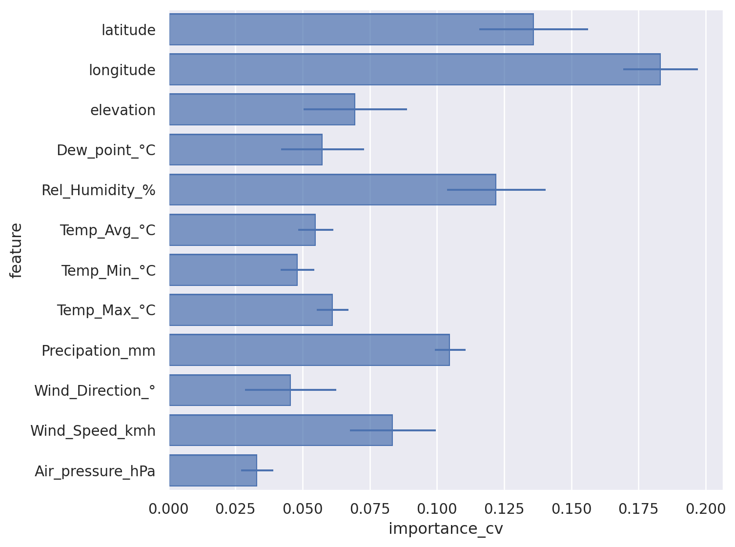
Show importance as bar chart including errorbars

Trick: flip x and y axis for readibility

(
#!#    so.Plot(feature_importances_long,x=??,y=??)
    so.Plot(feature_importances_long,x='importance_cv',y='feature')
    .add(so.Bar(), so.Agg())				## Bar plot showing the average
	.add(so.Range(), so.Est(errorbar="sd"))	## Whiskers showing the standard deviation
	.layout(size=(8, 6))	
)

There are problems with bar charts and errorbars: https://doi.org/10.1371/journal.pbio.1002128

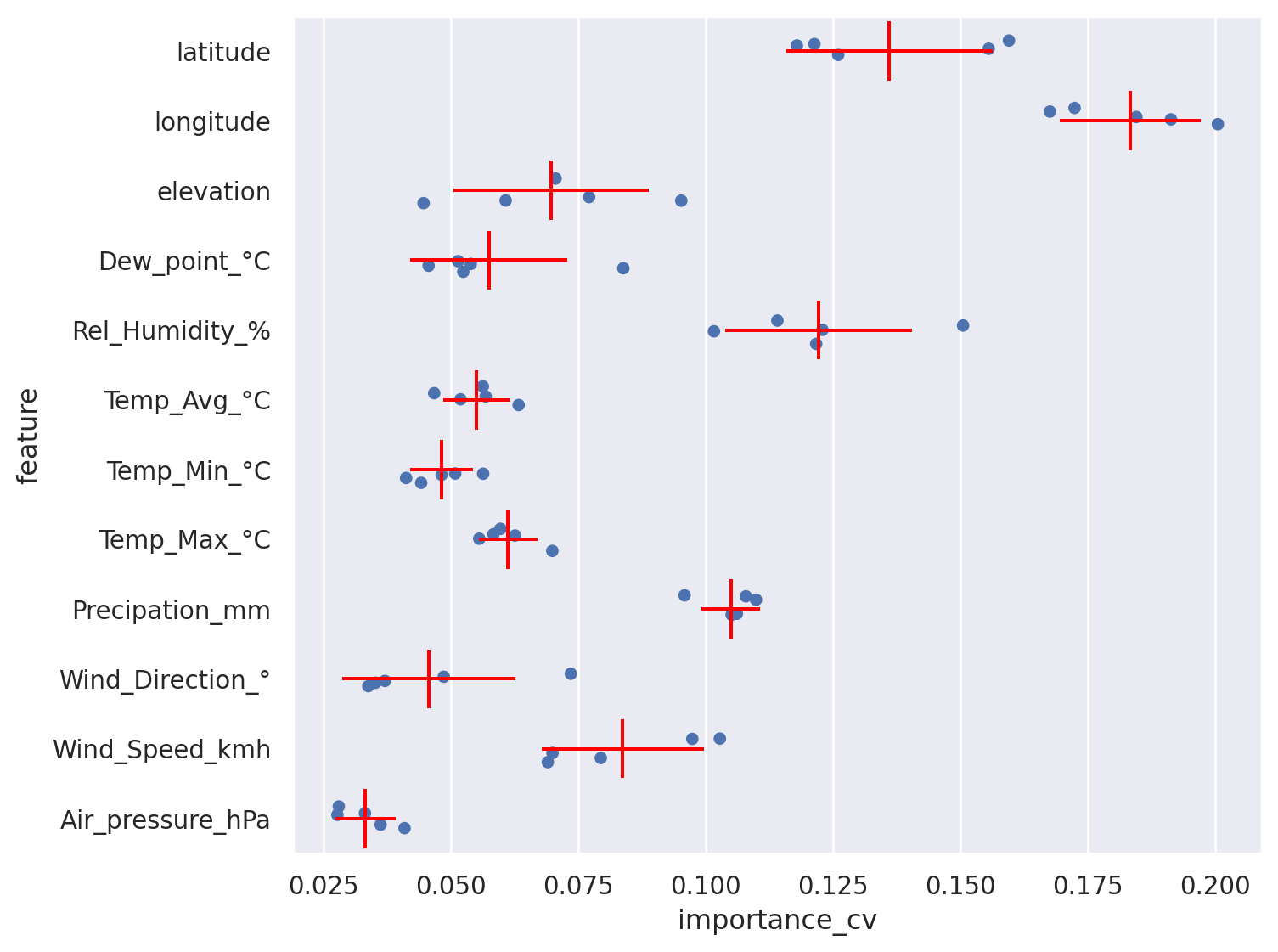
Better show points/dots for every trained model (sample) and statistics

(
    so.Plot(feature_importances_long,x='importance_cv',y='feature')
	.add(so.Dot(pointsize=5), so.Shift(y=.0), so.Jitter(.5)) ## Jitter and Shift avoid overplotting
#!# .add(so.??(color="red"), so.Agg())					## Show a dash with the average
#!# .add(so.??(color="red"), so.Est(errorbar="sd"))		## Show the range of the standard deviation 
    .add(so.Dash(color="red"), so.Agg())					## Show a dash with the average
	.add(so.Range(color="red"), so.Est(errorbar="sd"))		## Show the range of the standard deviation
	.layout(size=(8, 6))	
)